Dynamic Force Analysis Intro
Dynamic Force Analysis (commonly called DFA) is closely connected to PVA Analysis. After obtaining the motion of a system through PVA analysis, DFA obtains the forces acting on each link and joint in the system. This process of going from a known motion to the forces that would have caused such motion is called inverse kinematics. This is opposed to forward kinematics, where the motion of a system is determined given the external loading. In real life applications, both methods are used to analyze mechanisms.
Most of the time, the largest loads will be external forces and torques, as well as inertial forces and torques. To simplify our analysis, we will neglect the influence of gravity. However, in cases where gravitational loads contribute significantly to the total loads on a system, it is important to include them.
Review of Dynamics Concepts
There are a couple of applicable dynamics concepts that are worth reviewing.
Total mass tells us the resistance of an object to changes in linear acceleration given an external force. We can use Newton's second law to relate force, mass, and linear acceleration.
Center of mass is the first moment of mass. This is essentially the weighted sum of masses times their distances from a reference point. For a discrete set of point masses, we can use summation.
For continuous objects, we integrate over the entire volume to calculate the weighted sum.
In practice, the center of mass of many common shapes has already been solved and tabulated in look-up tables. Such tables can be readily found online or in textbooks. If the object is placed in a uniform gravitational field, then the object's center of gravity will be at the same location. Additionally, a free object will always rotate about an axis that goes through its center of mass. Additional information about centers of mass, and a table of centers of masses for common objects is located on the Rigid Body Kinetics page.
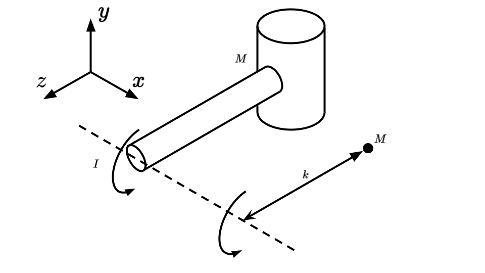
Moment of inertia is the second moment of mass. This tells us about an object's resistance to changes in angular acceleration. An object's moment of inertia is always considered around an axis of rotation. For example, the z-axis moment of inertia of a planar object can be calculated as such:Similar to the center of mass, the moment of inertia of common shapes about an object's center of mass have already been solved around the \( x \), \( y \), and \( z \) axes and tabulated. Additional information about moments of inertia of mass, and a table of moments of inertia for common objects is located on the Rigid Body Kinetics page.
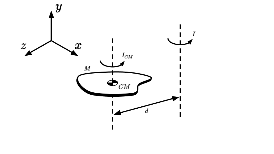
The parallel axis theorem allows us to calculate the moment of inertia of an object about any axis away from the center of mass. Objects rarely rotate around their center of mass in reality, especially when the object is part of a linkage. As such, having a method to calculate an object's moment of inertia about an arbitrary axis (without redoing the integral) is useful. The parallel axis theorem states that given the moment of inertia, \( I_{CM} \), about an axis through the center of mass of an object of mass \( M \), the moment of inertia about a parallel axis that is distance \( d \) away from the center of mass is given by:
The cross product is a useful mathematical operation that takes two vectors as input and returns a vector as output, denoted by the \( \times \) operator. Qualitatively, the magnitude of \( \vec{a}\times\vec{b} \) has the same length as the area of the parallelogram formed by \( \vec{a} \) and \( \vec{b} \), and the direction is determined by the right hand rule. Point your right hand's index finger in the direction of \( \vec{a} \) and the middle finger in the direction of \( \vec{b} \), then straightening your thumb will give the direction of \( \vec{a}\times\vec{b} \). This also shows that the cross product is not communicative, i.e., \( \vec{b}\times\vec{a}=-(\vec{a}\times\vec{b}) \).
Quantitatively, we have two methods to easily calculate the magnitude of the cross product of two 2D vectors, \( \vec{a}=a_x\hat{i}+a_y\hat{j} \) and \( \vec{b}=b_x\hat{i}+b_y\hat{j} \). The first method takes the determinant of a matrix containing the components of \( \vec{a} \) and \( \vec{b} \), as shown below:
The second method calculates the area of the parallelogram bounded by \( \vec{a} \) and \( \vec{b} \), where \( \theta \) is the angle between \( \vec{a} \) and \( \vec{b} \):
3D cross products are more challenging and require solving the determinant shown below. This is less useful in the context of DFA, since most linkages studied here operates in a plane.
Note that setting \( a_z=b_z=0 \) will yield the same result as the 2D case.
DFA procedure
Because we are dealing with multiple links, each applying forces and having forces applied onto it, we need a way to keep track of all the various forces. As such, the following notation will be used:
- \( \vec{F}_{ij} \): Force link \( i \) exerts on link \( j \). From Newton's Third Law, \( \vec{F}_{ij}=-\vec{F}_{ji} \).
- \( T_{ij} \): Torque link \( i \) exerts on link \( j \). Fron Newton's Third law, \( T_{ij}=-T_{ji} \).
- \( \vec{R}_{ij} \): Position of \( \vec{F}_{ij} \) relative to the CG of link \( j \). Note that unlike forces, \( \vec{R}_{ij}\neq\vec{R}_{ji} \) for this notation.
Here is a brief overview of the DFA procedure:
- Draw the complete system. Label points, dimensions, external forces and torques, and kinematics.
- Create free-body diagram for each segment. Each free-body diagram should include a labeled coordinate system, external joint forces and torques, kinematics, internal forces and torques, and position vectors. It is highly recommended to follow the notation shown above for ease of bookkeeping.
- Symbolically write out equations of motion for each link. For planar mechanisms, this will involve two force equations and one torque equation, for a total of three equations of motion:
- Convert equations to matrix format \( [A]\{B\}=\{C\} \) .
- Matrix \( [A] \) contains all geometric information (e.g. position vectors).
- Vector \( \{B\} \) contains all unknown forces and torques.
- Vector \( \{C\} \) contains all dynamic information (e.g. external forces and torques, PVA analysis results, mass, moments of inertia).
- Insert known values into the matrix equation.
- Invert matrix \( [A] \) to solve for \( \{B\} \) using a computational tool of your choice (e.g. MATLAB or Python).
DFA Walkthrough
Let's first apply DFA on a simple two-link system to see how it works. Link 1 is the ground link, while link 2 rotates around point \( O_2 \) and is acted on by an external force \( \vec{F}_P \). Link 2 has mass \( m \), length \( l \), and a uniform cross section. We want to find the reaction force \( \vec{F}_{12} \) at \( O_2 \) and the driving torque \( T_{12} \).
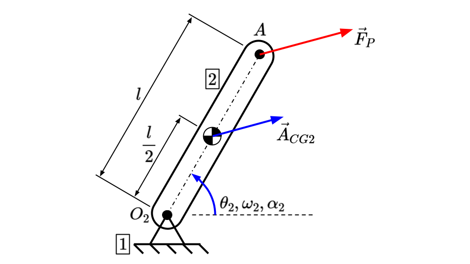
At this instant in time, the following parameters are known:
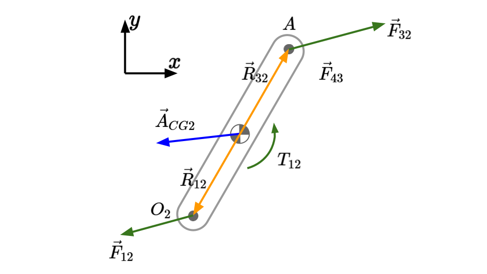
The equations of motion will be easier to visualize if we isolate link 2 and draw its free-body diagram:
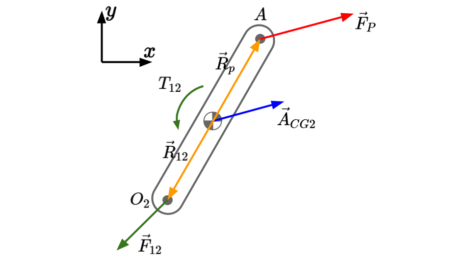
Writing out each equation of motion gives:
Next, group the known and unknown into \( [A] \), \( \{B\} \), and \( \{C\} \):
Putting the matrix equation together:
Substitute in all known values:
Invert and solve:
Now we can move on to a more complex example with multiple moving links. Below is a crank slider mechanism with an external force \( \vec{F}_p \) applied at point \( P \). A motor drives link 2. The slider (link 4) slides along a horizontal surface with friction coefficient \( \mu \). Assume that all kinematic and geometric information is known.
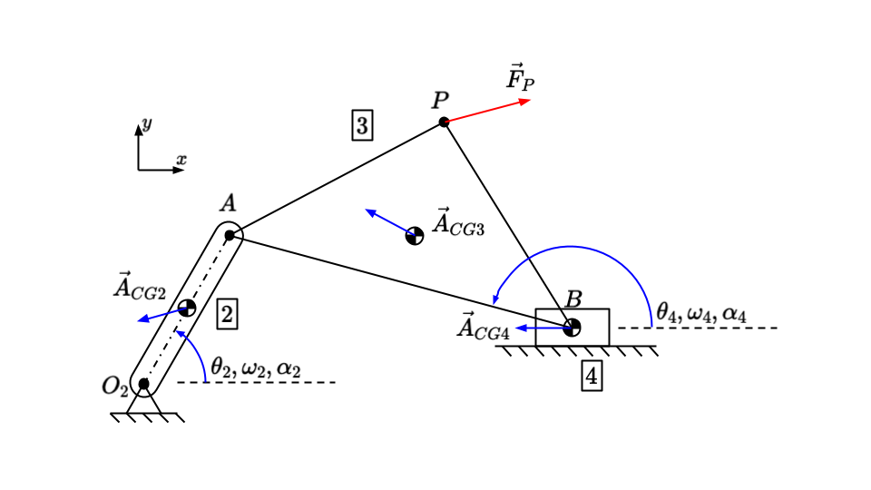
The unknowns are:
Note that we have the following redundant values:
Furthermore, we can use the friction coefficient to relate \( F_{14} \) and \( F_{14y} \). The sign of \( F_{14y} \) depends on the direction in which the slider is moving (that is, always opposite to the the velocity's direction).
Thus, we can reduce the unknowns down to 8 independent unknowns, which will require 8 equations to solve:
Next, draw the free body diagram for each link and write the respective equations of motion.
For link 2:
(Note that link 2 is identical to the link that was analyzed in the previous example.)
For link 3:
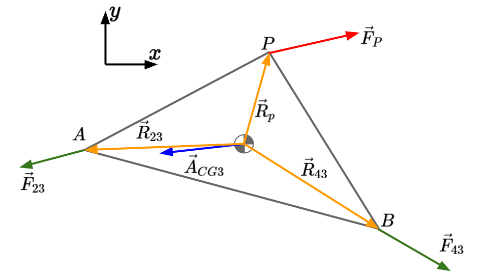
Recall that \( \vec{F}_{23}=-\vec{F}_{32} \).
For link 4:
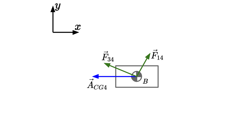
Note that torque balance is unnecessary because we assume that all forces are assumed to act through the CG.
We can now gather the 8 equations into matrix form \( [A]\{B\}=\{C\} \).
The final step is to solve for \( \{B\} \) by plugging in all known values, then taking the inverse of \( [A] \) and multiplying it by \( \{C\} \). i.e., \( \{B\}=[A]^{-1}\{C\} \).
Application Notes
If you have a mismatch between your number of equations and unknowns, there is likely a constraint on the problem that reduces the number of unknowns, or an equation that should not be included (sometimes this occurs with equations of the form \( 0=0 \)).