Rigid body kinetics
Euler's laws of motion
The laws of motion for rigid bodies were formulated by Leonhard Euler, which extended Newton's equations for point-masses to rigid bodies.
Euler's first law relates the mass \(m\) and acceleration of the center of mass \( \vec{a}_C \) of the body to the total force \( \vec{F} \) on the body (sum of all external forces). It describes the translational motion of the body.
Euler's second law relates the moment of inertia about the center of mass \(I_C\) and the angular acceleration of the body to the total moment \( \vec{M}_C \) (sum of all external moments) about the center of mass. It describes the rotational motion of the body.
Recall that the total force on a particle is related to the linear momentum of the particle. Thus, if we extend that to rigid bodies, we have an alternative way to express Euler's first law:
Similarly, the total moment on a particle about a certain point is related to the angular momentum of the particle about the same base point. We can do the same thing as above, and extend it to rigid bodies, and obtain an alternative form to Euler's second law:
Application alert!
Banked turns uses rigid body kinetics.
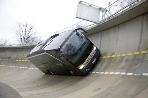
Rigid body kinetics can be used to analyze how vehicles move along banks.
Application alert!
Accelerating and braking uses rigid body kinetics.

Rigid body kinetics can be used to analyze how cars accelerate and brake.
Application Alert!
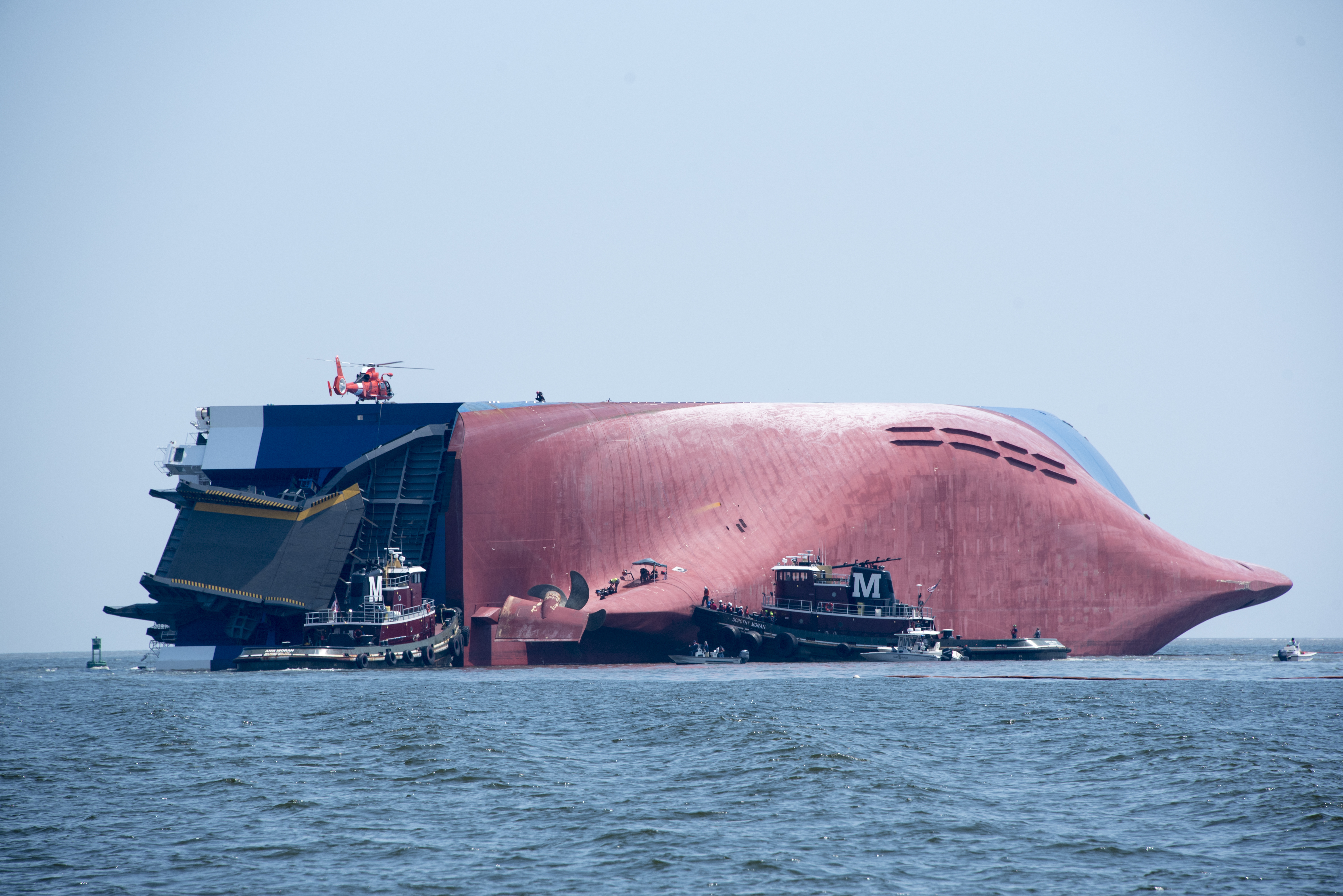
Ship stability uses Center of mass by ensuring the centers of gravity and bouyancy are in proper locations to avoid capsizing when out at sea.
Solution steps
The steps involved in analyzing a rigid body mechanical system with Newton's equations are as follows.
1. System diagram: The following is the system diagram for the pendulum. Use the polar coordinate system with theta defined as shown.

2. FBD: The following is the free body diagram for the pendulum.

The following forces are on the free body diagram.
3. Kinematics: \( \vec{a}_c, \vec{\alpha} \)
4. Kinetics: \( \sum \vec{F} = m \vec{a}_c, \sum M_{Cz} = I_{Cz} \alpha_z \) where \( c \) is the center of mass or \( \sum M_{Oz} = I_{Oz} \alpha_z \) where \( O \) is a fixed point.
Using \( \sum M_{Oz} = I_{Oz} \alpha_z \) makes it so that the force equation is not needed, since point \( O \) is fixed and therefore has no acceleration, which vastly simplifies the problem. The following steps can be used to take the moment about point \( O. \) From the FBD, \( r \) and \( F_{\theta} \) are perpendicular, so the following equation is true.
5. Algebra: