PVA Intro

Position, Velocity, Acceleration (PVA) analysis is used to analytically determine the motion of a mechanism. Position determines the configuration of the mechanism. Velocity is used to understand the kinetic energy and momentum of the system. Finally, acceleration is used to understand the forces in the system. PVA takes the known geometry, initial configurations, and PVA data of one link (the inputs) and determines the PVA data for the other links (the outputs).

Vector Calculus

In PVA analysis, links are represented using vectors. Using complex vectors is the easiest way to represent the link data as it utilizes the link length $|R|$ and starting link angle $\theta$ to create a vector. There are two forms of complex vectors that we will be focusing on: complex number form and polar form. Complex number form takes a Cartesian approach to complex numbers. Meanwhile polar form takes a polar approach (as the name suggests).

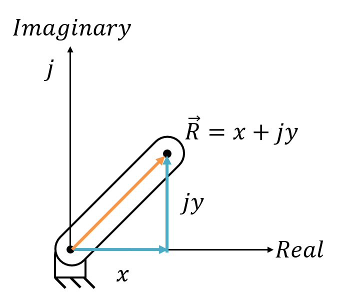
The $j$ in each vector represents the imaginary number \( sqrt{-1 \). The Euler formula can be used to break the polar form into the complex form.

Let's look at the polar vector form. Angle $\theta$ depends on time because the system is not static. This means that taking the derivative of the angle with respect to time will give the angular velocity $\omega$.

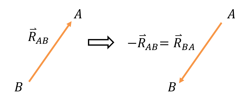
Also note that when you rotate a vector ${\overrightarrow{R}}_{AB}$ by 180 degrees, it becomes $-{\overrightarrow{R}}_{AB}$. Upon inspection, we can see that $-{\overrightarrow{R}}_{AB}$ is also equal to ${\overrightarrow{R}}_{BA}$. This can be a useful transformation to use when creating vector loops.

Vector Loops

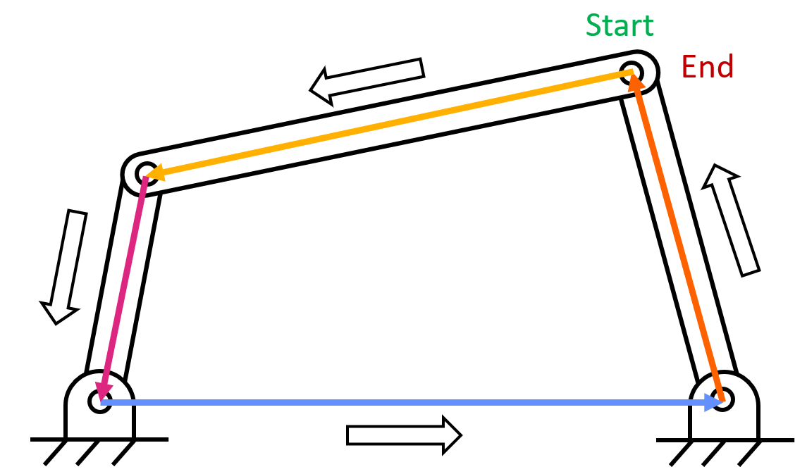
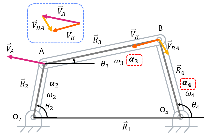
Vector loops are used to create equations that can be used to solve complex linkage problems. Vector loops work by creating a "loop" of vectors that start and end in the same location. This also means that the sum of these vectors is equal to zero. For example, take a look at a four bar linkage. If you choose a joint and trace around the links in one direction (making position vectors along the way) you end up creating a vector loop.

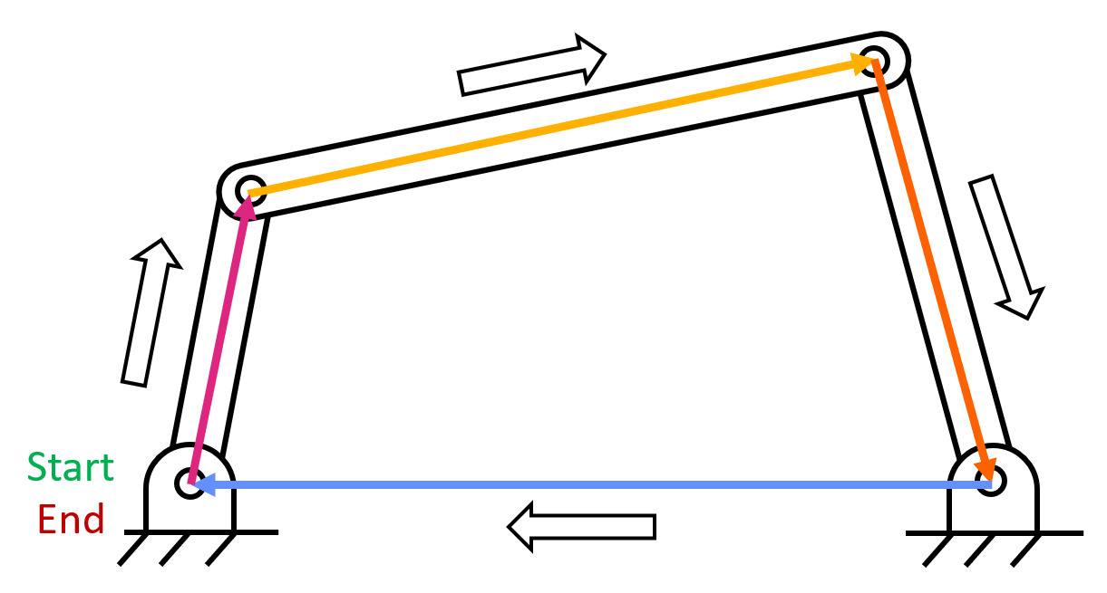
You can start the vector loop at any joint and go in any direction to finish the loop.

Alternatively, you can start at one point and go two different directions to end at a different point. As long as the two paths start and end at the same point, a vector loop can be created.

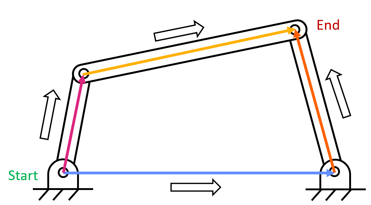
Since position, velocity, and acceleration are all path-independent vectors, we can usually write an equation in the form of ${\mathrm{\Sigma }}_0^n{\overrightarrow{R}}_n=0$. This gives us an equation we are able to solve.

Position Analysis

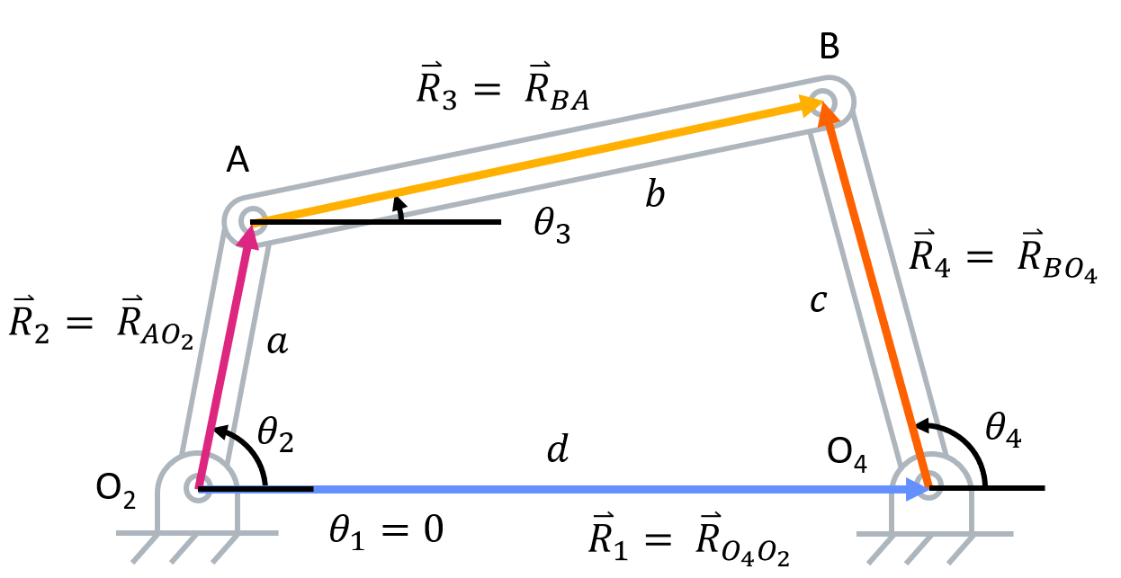
1. Identify known and unknown variables. In the four-bar linkage example, the linkage lengths ($a$, $b$, $c$, and $d$) and the initial angle of the crank $({\theta }_2)$ is known. The angle of the grounded link $({\theta }_1)$ is known to be zero. The initial angle of the coupler $({\theta }_3)$ and rocker $({\theta }_4)$ are unknown.

2. Establish a vector loop and write out the vectors in polar form. Recall that the polar form of a vector is in the form of $\overrightarrow{R}=|R|e^{j\theta }$. Since the vector loop we established uses two different paths to get from the same starting point to the same ending point, we have to set the sum of the two paths equal to each other.

Position Vector Loop Equations
$$\begin{array}{c}{\overrightarrow{R}}_2+{\overrightarrow{R}}_3={\overrightarrow{R}}_4+{\overrightarrow{R}}_1\\ {\overrightarrow{R}}_2+{\overrightarrow{R}}_3-{\overrightarrow{R}}_4-{\overrightarrow{R}}_1=0\\ {\overrightarrow{R}}_{A{O}_2}+{\overrightarrow{R}}_{BA}-{\overrightarrow{R}}_{B{O}_4}-{\overrightarrow{R}}_{O_4{O}_2}=0\\ a{e}^{j{\theta }_2}+b{e}^{j{\theta }_3}-c{e}^{j{\theta }_4}-d{e}^{j{\theta }_1}=0\end{array}$$
3. Break vector loop equation into real and imaginary parts. This can be done by using the Euler formula above.
   Position Vector Loop Equations in Cartesian Form

   $$\begin{array}{c}a{e}^{j{\theta }_2}+b{e}^{j{\theta }_3}-c{e}^{j{\theta }_4}-d{e}^{j{\theta }_1}=0\\ a(cos{\theta }_2+jsin{\theta }_2)+b(cos{\theta }_3+jsin{\theta }_3)-c(cos{\theta }_4+jsin{\theta }_4)-d(cos{\theta }_1+jsin{\theta }_1)=0\end{array}$$
   Remember that ${\theta }_1$ is equal to zero. This means that $d(cos{\theta }_1+jsin{\theta }_1)$ simplifies to just $d+0j$. Now we can easily break up the vector loop equation into its real and imaginary components.
   Real Component

   $$a(cos{\theta }_2)+b(cos{\theta }_3)-c(cos{\theta }_4)-d=0$$
   Imaginary Component

   $$a(sin{\theta }_2)+b(sin{\theta }_3)-c(sin{\theta }_4)+0=0$$
4. Solve for unknown positions and/or angles. Since lengths $a$, $b$, $c$, and $d$ are given along with angles $({\theta }_1)$ and $({\theta }_2)$, the unknowns are $({\theta }_3)$ and $({\theta }_4)$. Since there are two equations and two unknowns, this system can be solved using an equation solver.

Velocity Analysis

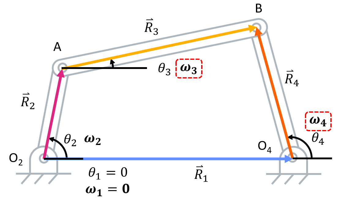
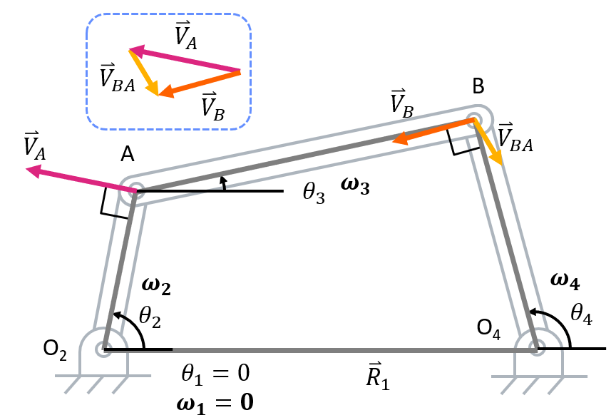
1. Identify known and unknown variables. All of the variables found in position analysis are known (including $({\theta }_3)$ and $({\theta }_4)$ as those were solved for in the last step of position analysis). In addition to these variables, ${\omega }_2$ is given. This leaves us with ${\omega }_3$ and ${\omega }_4$ as unknowns. Also, recall the position vector loop.
   Position Vector Loop

   $$a{e}^{j{\theta }_2}+b{e}^{j{\theta }_3}-c{e}^{j{\theta }_4}-d=0$$
   
2. Take the time derivative of the position vector loop to get the velocity vector loop.
   Velocity Vector Loop Equations

   $$\begin{array}{c}\frac{d}{dt}(a{e}^{j{\theta }_2}+b{e}^{j{\theta }_3}-c{e}^{j{\theta }_4}-d{e}^{j{\theta }_1})=0\\ ja\frac{d{\theta }_2}{dt}{e}^{j{\theta }_2}+jb\frac{d{\theta }_3}{dt}{e}^{j{\theta }_3}-jc\frac{d{\theta }_4}{dt}{e}^{j{\theta }_4}-jd\frac{d{\theta }_1}{dt}{e}^{j{\theta }_1}=0\end{array}$$

   Because linkage 1 is grounded, we also know that $\frac{d{\theta }_1}{dt}={\omega }_1=0$

   Simplified Vector Loop Equation

   $$j{\omega }_{2}a{e}^{j{\theta }_2}+j{\omega }_{3}b{e}^{j{\theta }_3}-j{\omega }_{3}c{e}^{j{\theta }_4}=0$$

   Or more specifically,

   Reduced Vector Loop Equation

   $${\overrightarrow{V}}_A+{\overrightarrow{V}}_{BA}-{\overrightarrow{V}}_B=0$$

   In this velocity vector loop ${\overrightarrow{V}}_{AB}$ represents the velocity of joint $B$ with respect to $A$.

   
3. Break vector loop equation into real and imaginary parts.
   Velocity Vector Loop Equations in Cartesian Form

   $$\begin{array}{c}j{\omega }_{2}a{e}^{j{\theta }_2}+j{\omega }_{3}b{e}^{j{\theta }_3}-j{\omega }_{3}c{e}^{j{\theta }_4}=0\\ j{\omega }_{2}a(cos{\theta }_2+jsin{\theta }_2)+j{\omega }_{3}b(cos{\theta }_3+jsin{\theta }_3)-j{\omega }_{3}c(cos{\theta }_4+jsin{\theta }_4)=0\end{array}$$
   Real Component

   $$-a{\omega }_{2}sin({\theta }_2)-b{\omega }_{3}sin({\theta }_3)+c{\omega }_{4}sin({\theta }_4)=0$$
   Imaginary Component

   $$a{\omega }_{2}cos({\theta }_2)+b{\omega }_{3}cos({\theta }_3)-c{\omega }_{4}cos({\theta }_4)=0$$
4. Solve for the unknown velocities. Using trigonometric identities, we can use the two above equations to solve for ${\omega }_3$ and ${\omega }_4$ using an equation solver.
+
Warning: Computing Velocities #warn1
Note that it is possible to solve for for ${\omega }_3$ and ${\omega }_4$ analytically. However this can be time consuming and depends on the exact nature of the mechanism that is being analyzed. For a standard 4-bar linkage with pin joints the solution is:
Velocity Solutions for 4-bar Linkage with Pin Joints
$$\begin{array}{c}{\omega }_3=\frac{a{\omega }_{2}sin({\theta }_4-{\theta }_2)}{bsin({\theta }_3-{\theta }_4)}\\ {\omega }_4=\frac{aomeg{a}_{2}sin({\theta }_2-{\theta }_3)}{bsin({\theta }_4-{\theta }_3)}\end{array}$$

Acceleration Analysis

1. Identify known and unknown variables. In addition to the known values from the position and velocity analyses, ${\alpha }_2$ is given. That leaves ${\alpha }_3$ and ${\alpha }_4$ as unknowns. Also, recall the velocity vector loop.
Velocity Vector Loop
$$j{\omega }_{2}a{e}^{j{\theta }_2}+j{\omega }_{3}b{e}^{j{\theta }_3}-j{\omega }_{3}c{e}^{j{\theta }_4}=0$$

2. Take time derivative of velocity vector loop to get acceleration vector loop.
   Acceleration Vector Loop Equations

   $$\begin{array}{c}\frac{d}{dt}(j{\omega }_{2}a{e}^{j{\theta }_2}+j{\omega }_{3}b{e}^{j{\theta }_3}-j{\omega }_{3}c{e}^{j{\theta }_4})=0\\ \\ j\frac{d{\omega }_2}{dt}a{e}^{j{\theta }_2}+j^2{\omega }_2\frac{d{\theta }_2}{dt}a{e}^{j{\theta }_2}+j\frac{d{\omega }_3}{dt}b{e}^{j{\theta }_3}+\\ j^2{\omega }_3\frac{d{\theta }_3}{dt}b{e}^{j{\theta }_3}-j\frac{d{\omega }_3}{dt}c{e}^{j{\theta }_4}-j^2{\omega }_4\frac{d{\theta }_4}{dt}c{e}^{j{\theta }_4}=0\\ \\ j{\alpha }_{2}a{e}^{j{\theta }_2}-{\omega }_2^{2}a{e}^{j{\theta }_2}+j{\alpha }_{3}b{e}^{j{\theta }_3}-{\omega }_3^{2}b{e}^{j{\theta }_3}-j{\alpha }_{4}c{e}^{j{\theta }_4}+{\omega }_3^{2}c{e}^{j{\theta }_4}=0\end{array}$$

   Now we can see terms with $\alpha$ and ${\omega }^2$ appearing for each linkage. The angular acceleration term $\alpha$ appears due to tangential, acceleration of the linkage while the ${\omega }^2$ term appears due to the centripetal acceleration of the linkage. In total, four different types of acceleration can appear in acceleration analysis. For a refresher on these terms, refer to the particle kinematics page on the dynamics reference page. With this information, we can simplify the equation further to focus on the different acceleration terms:

   Simplified Acceleration Loop Equation

   $$(j{\alpha }_2{\overrightarrow{R}}_2-{\omega }_2^2{\overrightarrow{R}}_2)+(j{\alpha }_3{\overrightarrow{R}}_3-{\omega }_3^2{\overrightarrow{R}}_3)-(j{\alpha }_4{\overrightarrow{R}}_4-{\omega }_4^2{\overrightarrow{R}}_4)=0$$

   Or more specifically,

   Reduced Acceleration Loop Equation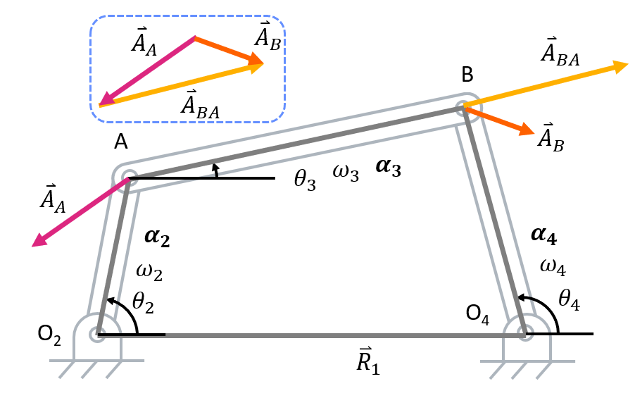

   $$\begin{array}{c}({\overrightarrow{A}}_A^t+{\overrightarrow{A}}_A^n)+({\overrightarrow{A}}_{BA}^t+{\overrightarrow{A}}_{BA}^n)-({\overrightarrow{A}}_B^t+{\overrightarrow{A}}_B^n)=0\\ {\overrightarrow{A}}_A+{\overrightarrow{A}}_{BA}-{\overrightarrow{A}}_B=0\end{array}$$
   
3. Break vector loop equation into real and imaginary parts.
   Acceleration Vector Loop Equations in Cartesian Form

   $$\begin{array}{c}j{\alpha }_{2}a{e}^{j{\theta }_2}-{\omega }_2^{2}a{e}^{j{\theta }_2}+j{\alpha }_{3}b{e}^{j{\theta }_3}-{\omega }_3^{2}b{e}^{j{\theta }_3}-j{\alpha }_{4}c{e}^{j{\theta }_4}+{\omega }_3^{2}c{e}^{j{\theta }_4}=0\\ \\ (j{\alpha }_2-{\omega }_2^2)a{e}^{j{\theta }_2}+(j{\alpha }_3-{\omega }_3^2)b{e}^{j{\theta }_3}-(j{\alpha }_4-{\omega }_4^2)c{e}^{j{\theta }_4}=0\\ \\ (j{\alpha }_2-{\omega }_2^2)a(cos{\theta }_2+jsin{\theta }_2)+(j{\alpha }_3-{\omega }_3^2)b(cos{\theta }_3+jsin{\theta }_3)-\\ (j{\alpha }_4-{\omega }_4^2)c(cos{\theta }_4+jsin{\theta }_4)=0\end{array}$$
   Real Component

   $$-a{\alpha }_{2}sin{\theta }_2-a{\omega }_2^{2}cos{\theta }_2-b{\alpha }_{3}sin{\theta }_3-b{\omega }_3^{2}cos{\theta }_3+c{\alpha }_{4}sin{\theta }_4+c{\omega }_4^{2}cos{\theta }_4=0$$
   Imaginary Component

   $$a{\alpha }_{2}cos{\theta }_2-a{\omega }_2^{2}sin{\theta }_2+b{\alpha }_{3}cos{\theta }_3-b{\omega }_3^{2}sin{\theta }_3-c{\alpha }_{4}cos{\theta }_4+c{\omega }_4^{2}sin{\theta }_4=0$$
4. Solve for the unknown accelerations. Using trigonometric identities, we can use the two above equations to solve for ${\alpha }_3$ and ${\alpha }_4$ using an equation solver.
+

Warning: Computing Accelerations #warn2

Note that it is possible to solve for for ${\alpha }_3$ and ${\alpha }_4$ analytically. However this can be time consuming and depends on the exact nature of the mechanism that is being analyzed. For a standard 4-bar linkage with pin joints the solution is:

${\alpha }_3=\frac{CD-AF}{AE-BD}$

${\alpha }_4=\frac{CE-BF}{AE-BD}$

Where

Acceleration Analytic Solution

$$\begin{array}{c}A=csin{\theta }_4\\ B=bsin{\theta }_3\\ C=a{\alpha }_{2}sin{\theta }_2+\alpha {\omega }_2^{2}cos{\theta }_2+b{\omega }_3^{2}cos{\theta }_3-c{\omega }_4^{2}cos{\theta }_4\\ D=ccos{\theta }_4\\ E=bcos{\theta }_3\\ F=a{\alpha }_{2}cos{\theta }_2-a{\omega }_2^{2}sin{\theta }_2-b{\omega }_3^{2}sin{\theta }_3+c{\omega }_4^{2}sin{\theta }_4\end{array}$$

While acceleration analysis is possible to do by hand, it is highly recommended that code or a computer based solver is used to assist solving for the unknown variables.

Application Notes

If you have more unknowns than equations, you can likely create more vector loops. If this is the case, think carefully about the constraints on your problems.

For example, take a look at this slider-crank example. If you create a position loop with three vectors, this leads to three unknowns (${\theta }_3$, $s(t)$, and $\beta (t)$).

By breaking up the position loop into four position vectors, it makes it clear that there are only two unknowns (${\theta }_3$ and $d(t)$).

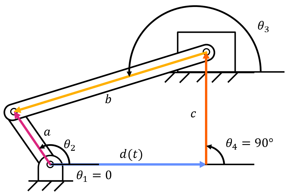
This leads to the following position vector loop:

Since ${\theta }_4$ equals 90 degrees and ${\theta }_1$ equals zero degrees, the equation can be simplified to:

When taking the time derivative of this equation, keep in mind that $d=d(t)$ is still a value that changes with respect to time. This will result in the terms $\dot{(}d)\ddot{(}d)$, which represents the change and rate of change in length of the link with respect to time.

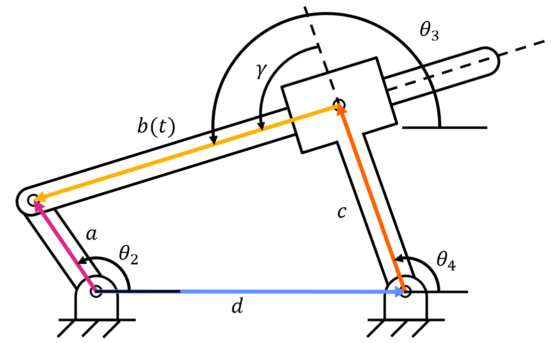
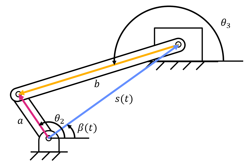
Similarly, if you set up a three-position vector loop for an inverted crank-slider, you will see three unknowns (${\theta }_3$, $s(t)$, and $\beta (t)$).

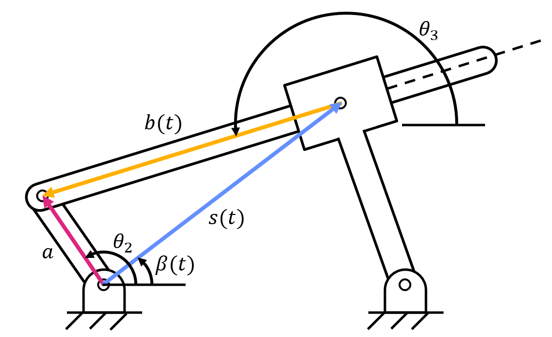
By breaking up the inverted crank-slider into four position vector loops, there are still three unknown variables (${\theta }_3$, $\beta (t)$, and ${\theta }_4$), but another equation appears due to geometry of the four-bar linkage. The angle $\gamma$ is constant because link four and the slider are fixed in an inverted crank-slider. This reveals the equation:

With three unknown variables and three equations, we can use a solver to obtain the values of all unknown variables.