Particle kinetics
Classical mechanics
Newton's equations relate the acceleration \( \vec{a} \) of a point mass with mass \( m \) to the total applied force \( \vec{F} \) on the mass (sum of all applied forces). They are:A point mass moving in the plane with an applied force. You can try to made the mass move in a circle and then see what happens when the force is suddenly removed, which will demonstrate Newton's first law (no net force implies motion at constant speed in a constant direction). Also observe which force directions cause the speed to increase or decrease.
Click and drag to impart a force on the particle.Did you know?
If we have objects which are either very massive, very small, or moving very fast, then Newton's equations do not provide a good model of their motion. Instead we must use Einstein's equations of general relativity (for massive and fast objects) or the equations of quantum mechanics (for very small objects). Unfortunately, these two theories cannot be used together, so we currently have no good models for objects which are simultaneously very small and very massive, such as micro black holes or the universe shortly after the big bang. Physicists are currently trying to reconcile general relativity with quantum mechanics by devising a new set of equations (sometimes called quantum gravity or a theory of everything). Current possibilities for new equations include string theory and loop quantum gravity, but none of these are generally accepted yet.
It is important to remember that all of these different equations are only models of reality and are not actually real:
“All models are wrong. Some models are useful.”
— George Box
Method of assumed forces and method of assumed motion
Newton's equations can be used in two main ways. Either we know the forces and we use this to compute the acceleration of a mass, or we know the acceleration and use this to compute the forces.Solution steps
The steps involved in analyzing a mechanical system with Newton's equations are as follows.A free-body diagram (abbreviated as FBD, also called force diagram) is a diagram used to show the magnitude and direction of all applied forces, moments, and reaction and constraint forces acting on a body. They are important and necessary in solving complex problems in mechanics.
What is and is not included in a free-body diagram is important. Every free-body diagram should have the following:
- The body represented as a dot if it is a point mass, and the body itself if it is a rigid body.
- The external forces/moments. The force vector should indicate: relative magnitude, point of application, and the direction.
- A properly defined coordinate system
A free-body diagram should not include the following:
- Bodies other than the body we are interested in.
- Forces applied by the body
- Internal forces depending on the chosen system. For example, a free-body diagram on a truss should not include the forces between individual truss members.
- Kinematic quantities (velocity and acceleration).
Warning!
Always assume the direction of forces/moments to be positive according to the appropriate coordinate system. The calculations from Newton/Euler equations will provide you with the correct direction of those forces/moments. Things that should not follow this are:
- Gravity
- Tension
- Friction if the velocity \( \vec{v} \) is provided
Warning!
If forces/moments are present, always begin with a free-body diagram. Do not write down equations before drawing the FBD as those are often simple kinematic equations, or Newton/Euler equations.
Numerical integration
- Independent variable (time).
- State variables come in pairs (position, velocity)(\( \theta , \omega \)).
- Initial conditions are the state variables at \( t=0 \).
- Time step \( \Delta t \) is how we jump forward in time.
- Update rule.
- Need to compute second derivatives (\( \ddot{\theta}=\alpha \) ) at each timestep.
Accelerating and braking
What happens when we step on the gas or brake in a car? The car pushes against the road to either accelerate (gas pedal) or decelerate (brake pedal). But how are the forces on the car and wheels distributed? What determines whether the wheels grip the road or lose traction and spin or slide?
To study this problem we need a model. Let's start with the simplest model and then gradually consider more complex models.
The simplest model of a car is to treat the entire vehicle as a point mass. On a we have vertical force balance for a stationary car. When the car , there is a horizontal forward force on the car, and a corresponding backwards horizontal force on the ground. As the car picks up speed, air resistance produces a backwards force. On the diagram we have drawn some forces offset from the center of mass, so that the vectors don't overlap. Because we are assuming a point mass model, however, all vectors are really acting at the same point.
While cruising at a constant speed, there is a balance between the horizontal driving force and the drag force due to air resistance. When the car , there is a backwards force that slows the car down to a stop.
We can think of the force vectors (such as the ground force on the car) as either in separate horizontal and vertical or as unified vectors. It may be helpful to pause the during and to consider the forces at work.
Reference material
Extra links
- Video of a burnout with a deliberate loss of traction.
- Video of a wheelie, where the front wheels lose contact.
- Video of braking in which the rear wheels lose contact.
- Another burnout video, taken to the point of destruction.
Banked turns
Turning in a circle requires a vehicle to have a centripetal acceleration inwards on the turn, and so there must be some centripetal force that produces this acceleration. For a vehicle driving on flat ground, this force must be produced by a sideways friction force on the tires. This introduces two problems:
- If the coefficient of friction is not high enough (say the road is wet or icy), then the friction force will be insufficient and the vehicle will slide off the road.
- Even if the friction force is high enough, because it acts at the bottom of the tires, it produces a net moment about the center of mass, which can cause the vehicle to roll over.
To avoid both of these problems, the road can be banked inwards, so that the outer edge of the road is higher than the inner edge. This is called superelevation and means that some of the centripetal force can be provided by the normal force with the road, reducing the friction force and minimizing the risk of slip or roll.
The figure below shows a bus driving around a sharp corner at high speed on a heavily banked road. To understand the dynamics of this vehicle and the design tradeoffs for cornering on banked turns, we need a model. We will start below with a simple point mass model, which will be enough to understand friction and sliding, and then move on to a 2D rigid-body body to understand roll behavior.
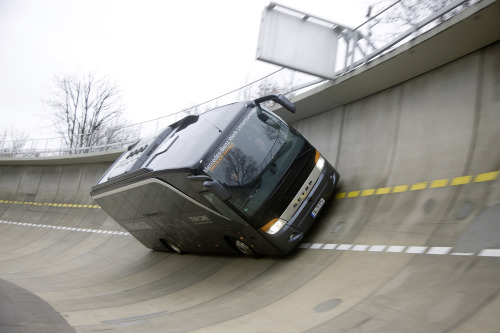
Setra S 411 HD coach from the TopClass 400 series on the Mercedes-Benz Untertürkheim test track. This 10.16 m long coach model is relatively compact and has short overhangs, allowing it to traverse the sharp banked corner at about 100 km/h. The vehicle is powered by an OM 501 LA V6-engine developing 300 kW (408 hp). Image source: Daimler Global Media Site (full-sized image).
Required material
- Kinetics of point masses
- Kinetics of rigid bodies
Extras!
- Video of a Dodge Challenger on the Untertürkheim track curve.
- Video of the bus shown in coach figure.
- Video taken from inside a car driving around the Untertürkheim track.
Track geometry
To understand the dynamics of the bus above, we first need a simple model of the geometry of the road. A satellite photo of the track is shown below. The bus was photographed while on the far-left-hand curve, which we can see is approximately a half-circle with radius about 50 m.
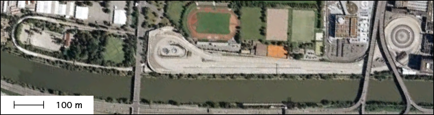
Satellite image of the Mercedes-Benz test track at Untertürkheim, on the Neckar River just outside of Stuttgart, Germany. The picture of the bus above was taken on the far-left-hand corner, which has a radius of curvature of about 50 m. Integrated with the test track is the excellent Mercedes-Benz Museum.
To make a simple model, let us consider a track with straight segments and half-circular ends, as shown below. If we the bus then we can see the for velocity, acceleration, and force as the bus drives around the track. We assume constant speed, so there is only an acceleration when the velocity changes direction around the corners. This model assumes semi-circular track ends, but this is not a good idea in practice.
The centripetal acceleration must be caused by an inwards force while going around the corners. To understand the magnitude and source of this force, we now consider a simple point mass model.
Did you know?
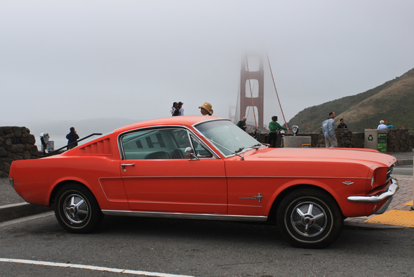
The modern automobile was invented in 1885 by Karl Benz in Mannheim, Germany, about 100 km from Stuttgart. The commercial success of the new invention was significantly aided by Benz' wife Bertha, who marketed the automobile by making the world's first road trip, inventing brake linings in the process. Driven by the post-WWI German economic crisis and hyperinflation, the Benz company later merged with Daimler to form Daimler-Benz, and began producing Mercedes-Benz cars in Untertürkheim, just outside of Stuttgart, where it is still headquartered. One of the company's engineers, Ferdinand Porsche, later founded his own company, which is also still based in Stuttgart.
Point mass model
Consider the bus as a single point mass on the track while going around the corner. The diagram below shows the bus front-on, so the inside of the track is towards the left. We start by assuming there is no bank on the road and that the bus is stationary. The shows that the gravity force \(W\) is balanced by the normal force \(N\) from the road. If we now increase the bank angle \(\theta\) below, then we see that a friction force \(F\) tangential to the road is needed to keep the bus from sliding. In practice, this force will be limited by \(F \le \mu N\), where \(\mu\) is the coefficient of friction. If we incline the track until it is nearly vertical, we see that there a huge friction force would be required but only a tiny normal force is available. As this would not be possible without gluing the tires to the road, this situation would result in the bus sliding downwards towards the center of the track.
Road bank angle:
Bus speed:
Now set the bank angle back to \(0^\circ\) and make sure the speed is zero and that the is visible. Now increase the speed of the bus to produce a centripetal acceleration. Newton's law implies that there must be a centripetal friction force producing this acceleration. As the speed increases, we will eventually reach a point when the friction force required is too large and the bus will slide outwards on the track.
To avoid sliding outwards, we can increase the bank on the road. This increases the normal force and decreases the friction force, making it less likely that sliding will occur. For any given speed, there is some angle that exactly cancels the friction force, so that all the force is normal force. This is a very safe driving situation, as no sliding is possible, even in very slippery road conditions. On the real track, the bank angle increases as the bus drives higher. This allows the driver to select the correct incline angle to minimize sliding risk. We can also show the forces in or as total vectors as we change the bank angle and bus speed.
While this simple point mass model allows us to understand how banking the road can help with the problem of sliding, it does not tell us anything about rolling of the vehicle, because point masses can't rotate. We thus need a rigid body model to investigate roll.
Did you know?
Higher speed and a smaller radius of curvature on a circular track requires higher bank angles, as in the photo below.
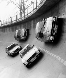
Mercedes-Benz models 450 SL and 450 SLC in the front, with models 450 SE and 450 SEL behind, on the Untertürkheim test track in 1973. Image credit: Daimler Global Media Site (full-sized image, original rotated image).
2D rigid body model
We now use a single rigid body model for the bus and we will do everything in 2D. Below we see a front-on diagram of the bus, with the inside of the track to the left. If we turn on the , then we see that the weight of the bus is supported by two forces, one on each wheel. If we increase \(\theta\) then the weight is supported more by the down-slope wheel, and we also see sideways friction forces appear to stop the bus from sliding. If the slope becomes too steep, then the normal force on the up-slope wheel reverses direction, indicating that it is holding the wheel down onto the road. Physically this cannot happen, so at this point the bus would tip over. We needed this rigid-body model to understand this tipping behavior, as we couldn't model this with the point mass model. Depending on the value of the friction coefficient, the bus may either slide or roll first as \(\theta\) increases.
Road bank angle:
Bus speed:
If we now set the bank angle \(\theta\) back to zero, we can start to increase the speed \(v\). Now we see that the wheel on the inside of the track takes less of the weight, and the friction forces now stop the bus from sliding outwards on the track. If the bus goes too fast then it will roll outwards on the track (assuming the friction coefficient is high enough that it didn't slide first).
Having considered both a banked road with stationary bus, and a moving bus on a horizontal road, we can now combine them to see the advantage of having a banked road when the bus is cornering. Choose a bus velocity, and then change the bank angle \(\theta\), so that the friction force is reduced (helping to avoid sliding) and the normal forces on the wheels are more evenly balanced (helping to avoid rolling). For any given speed, we can choose a bank angle so that there is simultaneously no sideways friction force and also exactly balanced normal forces. This is the safest bank angle for this speed.
Design of roads, tracks, and rail
A straight road generally has the center somewhat higher than the edges to allow water to run off. This is called cross slope or camber. When it is desired to have a banked turn, then the outer edge of the road is raised to produce superelevation, with the outer edge rising above both the center and the inner edge. The bank angle is chosen based on the radius of curvature of the turn and the expected speed of cars going around the turn, while still allowing for the fact that cars might be moving slowly or even stopped. The angle should thus not be chosen to eliminate all friction forces when cars are traveling at maximum speed, as this would be dangerous if traffic had to stop on the road.
Velodromes are arenas with tracks designed for high-speed bicycle races, as shown below, with speeds up to 85 km/h. The bank angle on velodrome tracks is chosen to minimize sideways forces on the bicycles when they are traveling at near maximum speeds, so the angle chosen depends on the radius of curvature of the track corners. For example, the Blaine velodrome track pictured below is 250 m long and has a 43° bank angle on the corners and 15° banking on the straightaways.
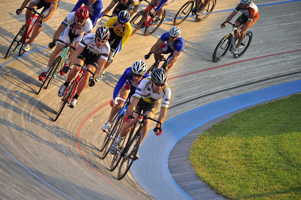
Bicycle riders on a banked turn at the Blaine velodrome, part of the National Sports Center in Blaine, Minnesota. Image source: flikr user flyinfoto (CC BY 2.0) (full-sized image).
High-speed trains such as the French TGV operate at speeds of over 300 km/h and have run at up to 575 km/h. To accommodate cornering at such speeds, track bends are constructed with a large radius of curvature (at least 7 km for new tracks) and a bank angle of up to about 7° (180 mm maximum superelevation with Standard gauge of 1435 mm). For railways, banking the track is know as cant.
An alternative approach for cornering with trains is to leave the track relatively flat and to tilt the train as it travels around a corner. This allows high-speed trains to operate on regular tracks, while maintaining safety and comfort for the passengers. For example, the Queensland Rail Tilt Train operates at 180 km/h by tilting at up to 5° around corners. As we see from our rigid body analysis above, tilting the train will help with avoiding tipping over at high speeds, but will not help with reducing horizontal friction forces. Even with a tilting train, entering a curve at too high a speed will lead to disastrous results.
Did you know?
The Blaine velodrome in Minnesota was designed by the famous Schuermann velodrome architects and built from the extremely durable African Afzelia hardwood. Velodrome races are always counter-clockwise and use special bikes with fixed chains (no freewheeling, no gears) and no brakes. The corners are scarily steep:
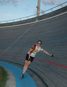
Image credit: Tom McGoldrick (full sized image).
Did you know?
High-speed trains such as the French TGV and German ICE require many sophisticated engineering techniques to enable travel at extreme speed. Very smooth rails are needed, so the track is formed by welding the segments together into one precisely-aligned continuous steel line. The steel rails conduct heat too well for conventional welding, so thermite welding is used to join the track segments.
At high speeds the train drivers are unable to see railway signals on the side of the track. Electronic signaling systems are used to communicate to the drivers, either through the tracks for the TGV or via additional cables for the ICE.
Friction-based brakes produce too much heat, as they would need to absorb the kinetic energy of several hundred tonnes of train moving at over 300 km/h. Instead, dynamic breaking is used, in which the electric motors powering the trains are run in reverse as generators and the energy is shed as heat in resistor arrays. At extremely high speeds, the wheels themselves cannot provide sufficient traction to enable braking, so technologies like magnetic induction brakes are being developed, which directly push against the rails without involving the wheels at all.
Bus model
The bus model used above is a Setra S 411 HD coach. The mass of the vehicle is 12.6 t and the dimensions are shown below.
| | |
Projectiles with air resistance
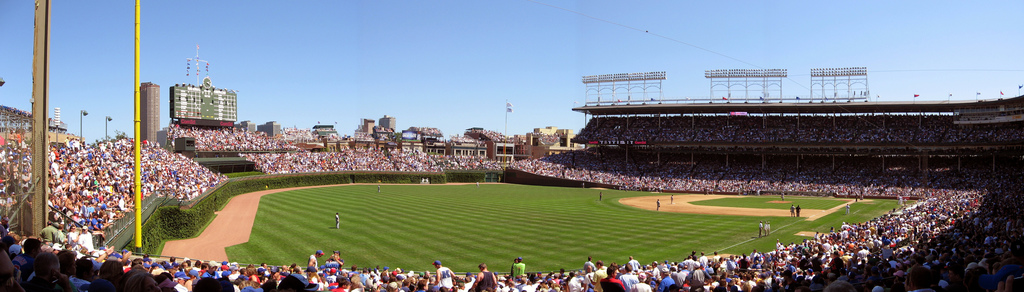
Consider a spherical object, such as a baseball, moving through the air. The motion of an object though a fluid is one of the most complex problems in all of science, and it is still not completely understood to this day. One of the reasons this problem is so challenging is that, in general, there are many different forces acting on such objects, including:
- gravity
- drag
- lift
- thrust
- buoyancy
- bulk fluid motion, such as wind
- inertial forces, such as the centrifugal and Coriolis forces
In most introductory physics and dynamics courses, gravity is the only force that is accounted for (this is equivalent to assuming that the motion takes place in a vacuum). Here we will consider realistic and accurate models of air resistance that are used to model the motion of projectiles like baseballs.
Drag forces and drag coefficients
The drag force is always directly opposed to the velocity of the object. In vector notation,
Velocity angle from horizontal:
The free body diagram for a baseball subject to gravity and air resistance. Observe that the drag due to air resistance is always in the opposite direction to the velocity. Image credit: Microsoft clip art.
The magnitude of the drag force is characterized by the dimensionless drag coefficient \( C_{\rm D} \), given by
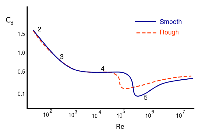
Drag coefficients as a function of Reynolds number
A dimensionless parameter that is very useful in fluid dynamics is the Reynolds number, which is defined as
An important result in fluid dynamics is that the drag coefficient is a function only of the Reynolds number of the fluid flow about the object. That is,
Quadratic drag model
Notice from Figure #aft-fd that there is a range of Reynolds numbers (\( 10^3 < {\rm Re} < 10^5 \)), characteristic of macroscopic projectiles, for which the drag coefficient is approximately constant at about 1/2 (see the part of the curve labeled “4” in Figure #aft-fd). That the drag coefficient is constant means that, within this region, the magnitude of the drag force is proportional to the square of the object’s speed. Substituting \( C_{\rm D}=1/2 \) into the definition of \( C_{D} \) above, we obtain
In the presence of gravity and quadratic drag alone, the net force on an object is given by
Initial speed:
Initial angle:
Mass:
Diameter:
Did you know?
There is no well-measured record for longest baseball home run. It is claimed that Mickey Mantle hit a ball 643 feet (196 m), although this apparently included rolling on the ground. Other power hits by Mantle are reliably measured to be over 500 feet (152 m).