Stress Transformation
General State of Stress
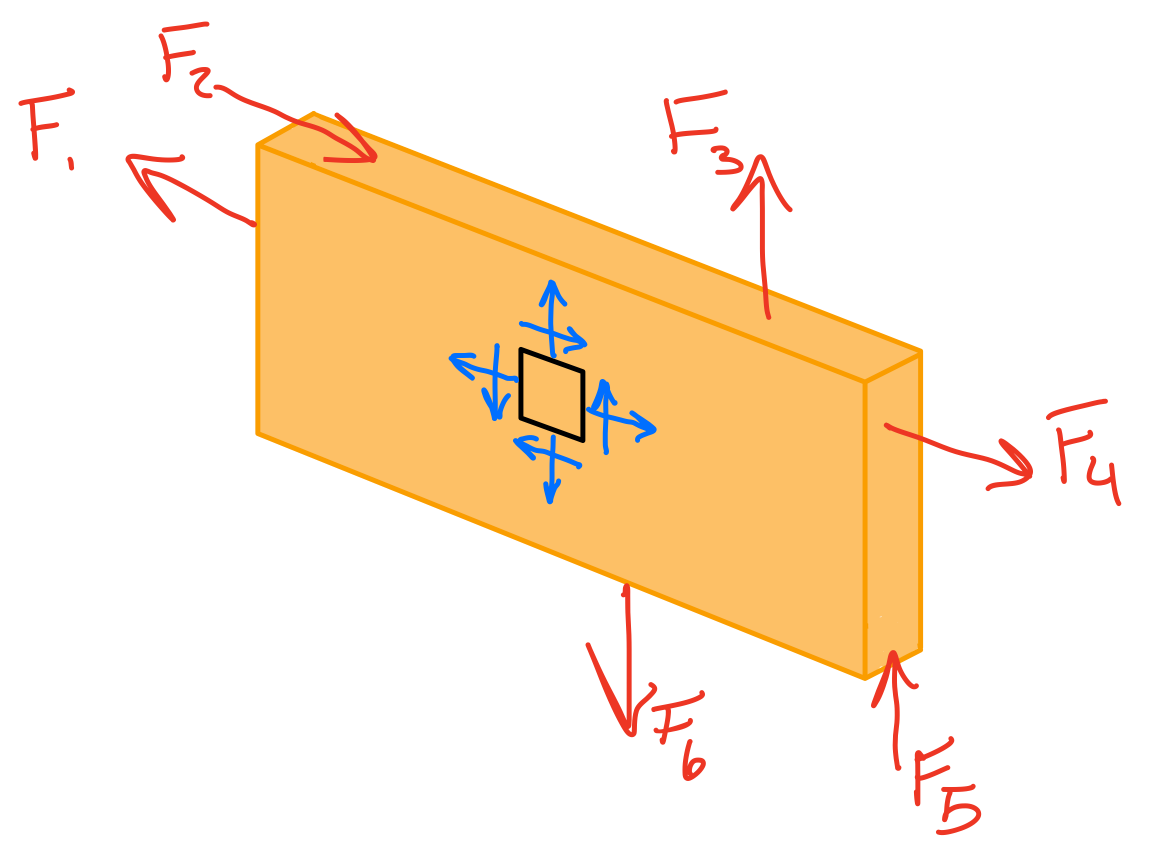
The general state of stress at a point is characterized by three independent normal stress components and three independent shear stress components, and is represented by the stress tensor. The combination of the state of stress for every point in the domain is called the stress field.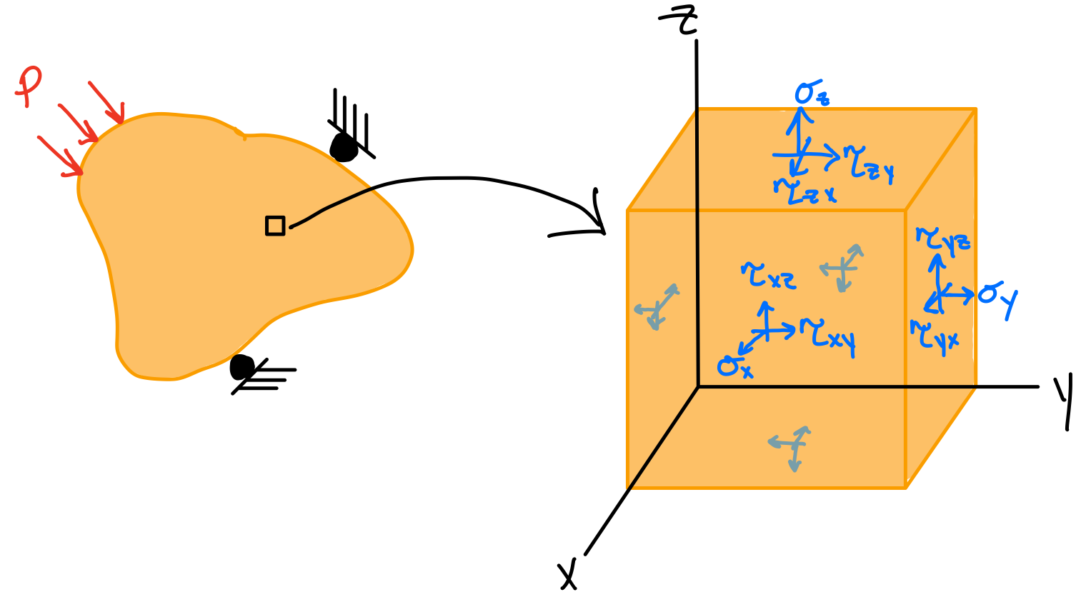
Sign Convention
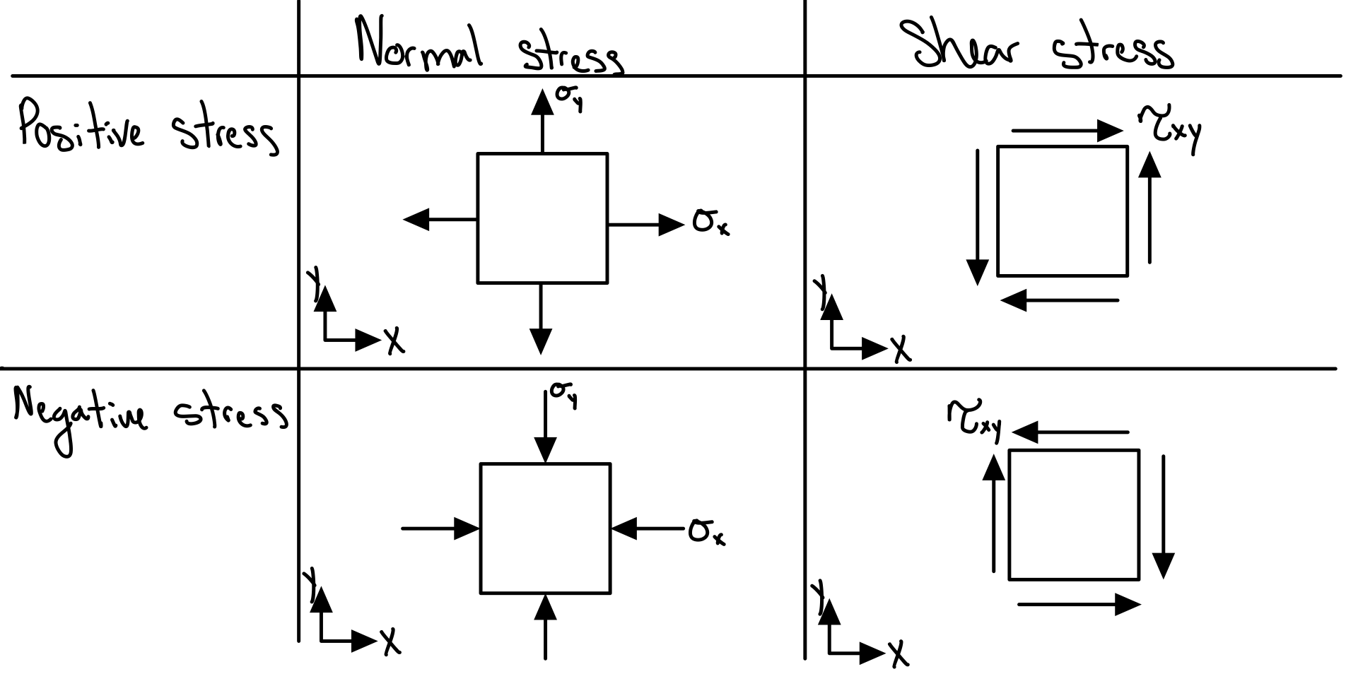
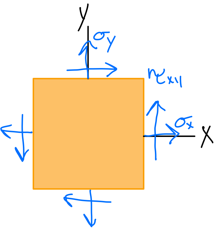
- Positive normal stress acts outward from all faces.
- Positive shear stress points towards the positive axis direction in a positive face.
- Positive shear stress points towards the negative axis direction in a negative face.
Plane Stress
Plane Stress Transformation
We think of stresses acting on faces, so we often associate the state of stress with a coordinate system. However, the selection of a coordinate system is arbitrary (materials don't know about coordinates - it's a mathematical construct!) and we could choose to express the stress state acting on any set of faces aligned with any coordinate system axes. Furthermore, we can relate the states of stress in each coordinate system to one another through stress transformation equations.
Heads up!
Cauchys stress theorem builds on this content in later solid mechanics courses.
For any surface that divides the body ( imaginary or real surface), the action of one part of the body on the other is equivalent to the system of distributed internal forces and moments and it is represented by the stress vector \( t^n \) (also called traction), defined on the surface with normal unit vector \( n \).
The state of stress at a point in the body is defined by all the stress vectors \( t^n \) associated with all planes (infinite in number) that pass through that point.
Transformation Sign Convention
- Both the \( x-y \) (original) and \( x’-y’ \) (transformed) systems follow the right-hand rule.
- The orientation of an inclined plane (on which the normal and shear stress components are to be determined) will be defined using the angle \( \theta \). The angle \( \theta \) is measured from the positive \( x \) to the positive \( x’ \) -axis. It is positive if it follows the curl of the right-hand fingers.
2-D Mohr's Circle
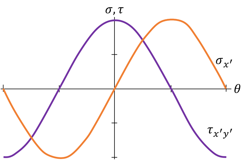
Mohr's circle is a graphical representation of stress transformations. The equations for stress transformations actually describe a circle if we consider the normal stress \( \sigma \) to be the x-coordinate and the shear stress \( \tau \) to be the y-coordinate.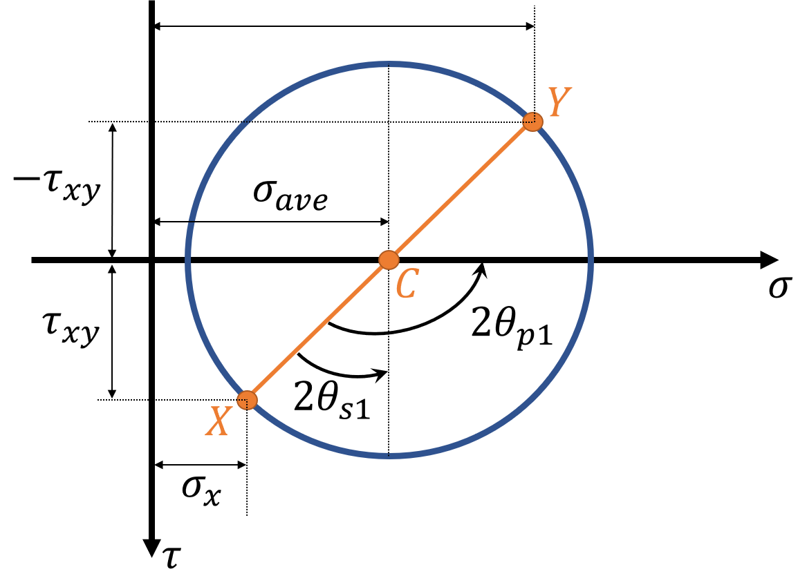
Interactive Mohr's circle
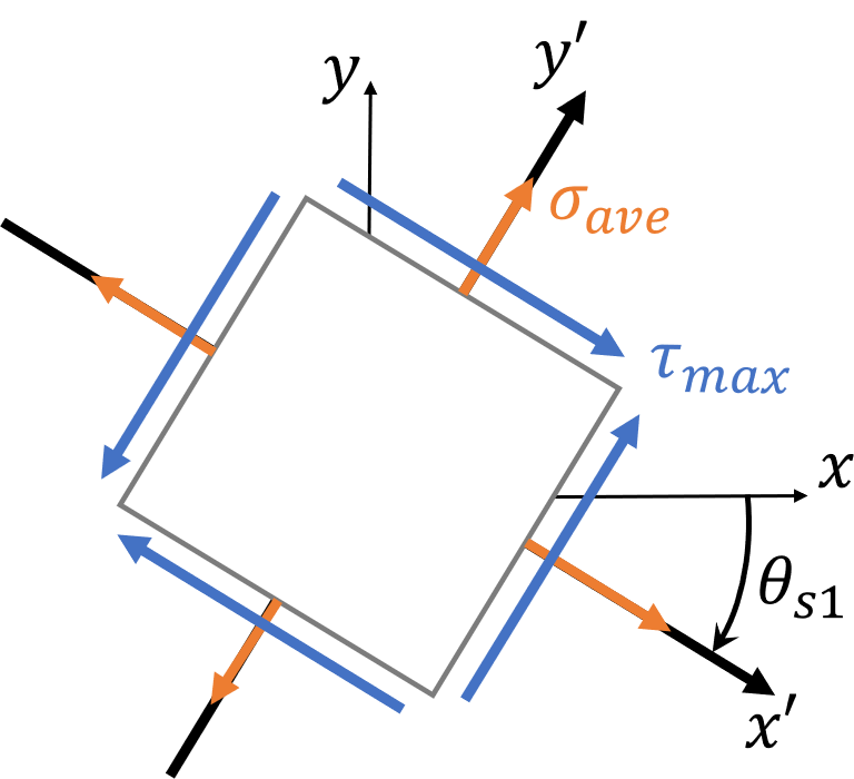
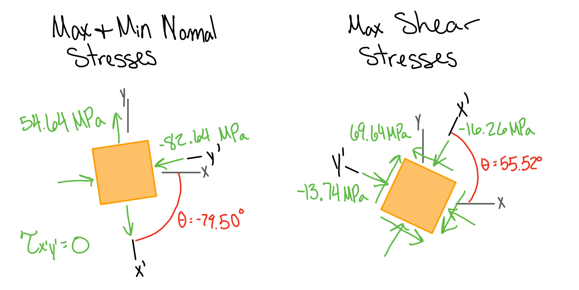
The stress element below is plotted on Mohr’s circle as shown in the left image. The right image shows the new orientation of the stress element.
Use the slider below to change the angle and see the corresponding angle for maximum normal stress and maximum shear stress.
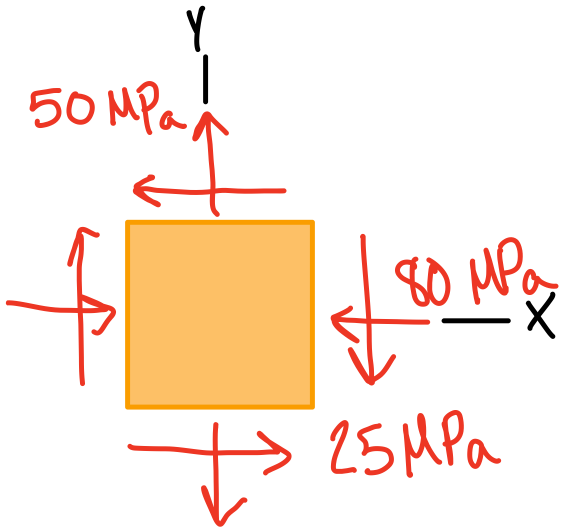
\( \sigma_x \): -80
\( \sigma_y \): 50
\( \tau_{xy} \): -25
\( \sigma_1 \):
\( \sigma_2 \):
\( \tau_{max} \):
\( \sigma_{x^{\prime}} \):
\( \sigma_{y^{\prime}} \):
\( \tau_{x^{\prime}y^{\prime}} \):
Angle:
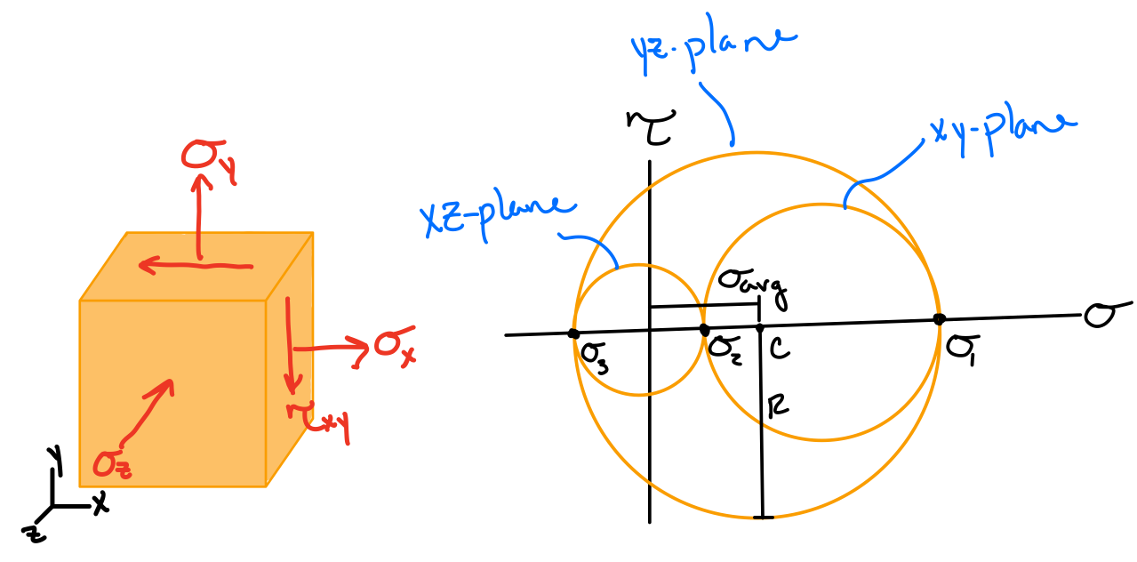
3-D Mohr's Circle
Stresses on Inclined Planes
Pure Shear
A circular shaft under torsion develops pure shear on cross-sections between longitudinal planes (the faces of element \( a \) are parallel and perpendicular to the axis of the shaft).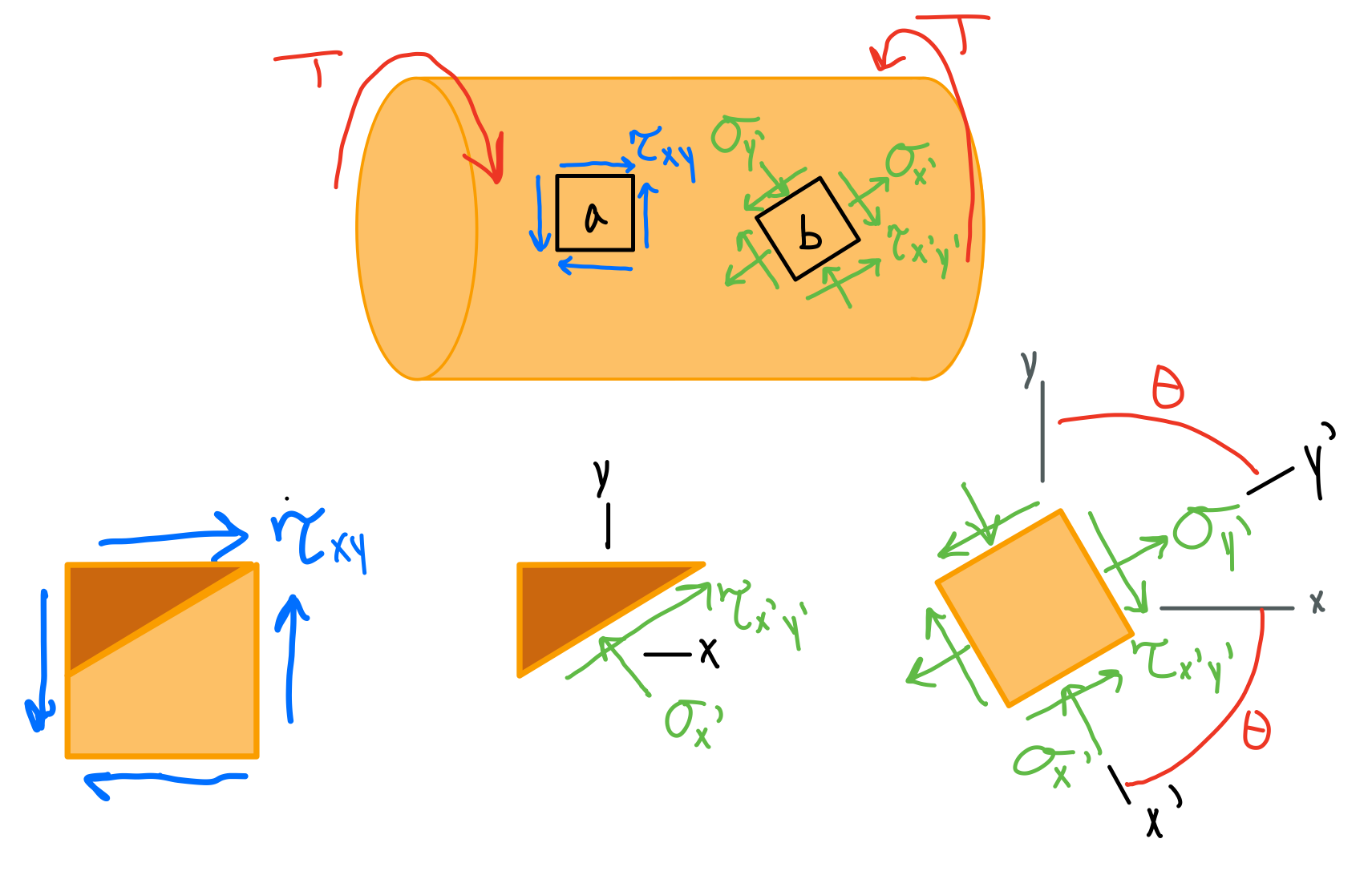
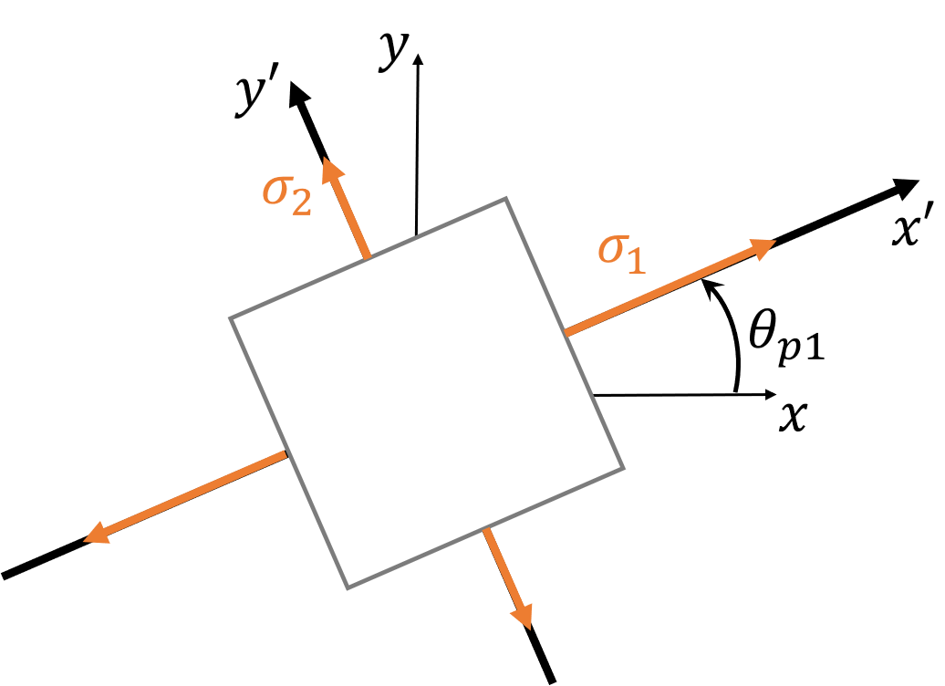
Principal Stresses
Alternative Approach: Eigenvalues
The eigenvalues of the stress tensor are called the principal stresses, and the eigenvectors define the principal direction vectors.Because of symmetry, the stress tensor (\( T \)) has real eigenvalues (\( \lambda \)) and mutually perpendicular eigenvectors (\( v \)).
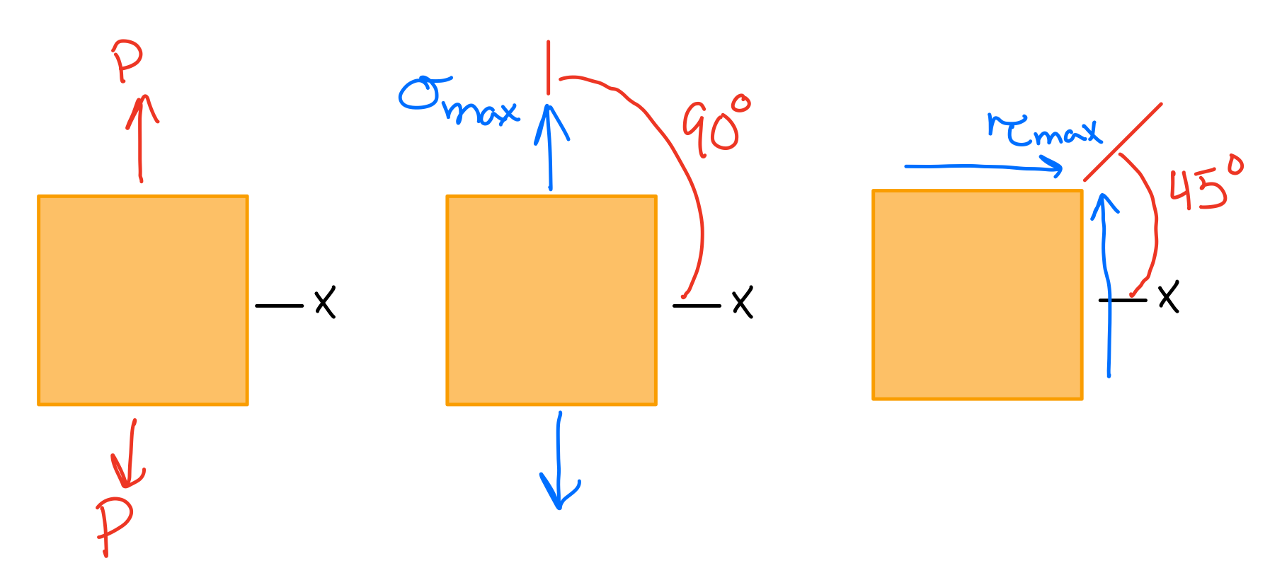
Maximum Shear Stress