Introduction to Cams

Cams are mechanical devices that allow a design to convert an input motion into pre-programmed output motion. A cam mechanism is comprised of two main components: the cam and the follower. The follower is in constant contact with the cam and, as the cam moves, it follows the geometry of the cam to produce an output motion.

Cams come in all shapes and sizes, resulting in many useful characterizations of their form and function. Cam geometries can be split into three categories:

• Radial - The follower's motion is perpendicular to the cam's axis of rotation.
• Cylindrical - The follower's motion is parallel to the cam's axis of rotation.
• Axial - The cam itself slides on a linear path.

Radial Cam

Cylindrical Cam

Axial Cam

Followers are ideally 1-DOF mechanisms. Two methods to restrict the follower's degree of freedom are:

• Rotating - The follower is restricted to rotate about an axis.
• Translating - The follower is restricted to slide inside a channel.

Figure 2: Follower Motion Types

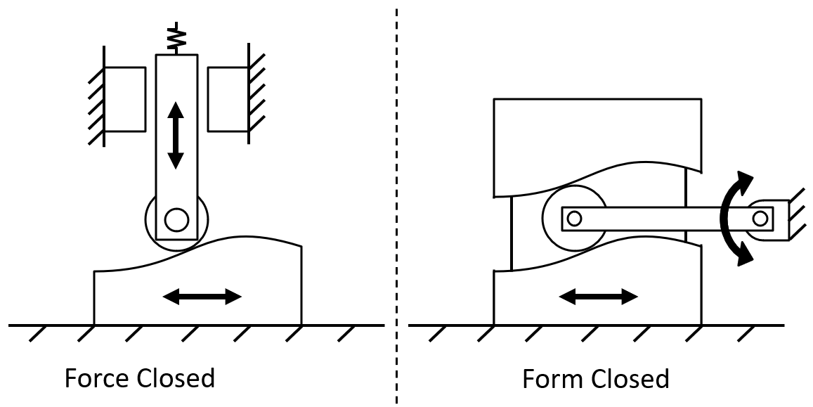
Followers must be in constant contact with the cam to ensure it follows the cam's geometry. Two methods of achieving constant contact are:

• Force closed - The follower is pressed into the cam by a force, e.g. from a spring or gravity.
• Form closed - The follower is held in place by the geometry of the cam.

Figure 3: Follower Closure Types

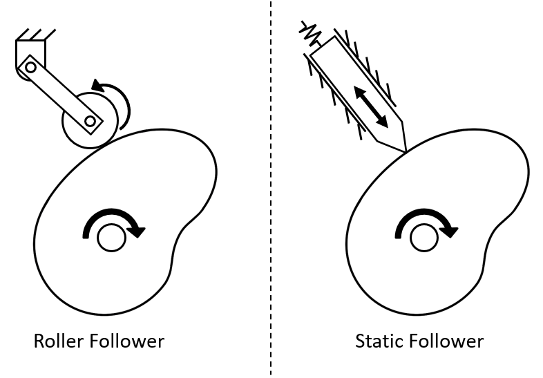
The point of contact between the follower and the cam is a major source of friction and wear, making the design of the follower is extremely important. The follower's shape can be generally placed in two categories:

• Roller - A small wheel on the follower rolls along the cam's profile. This has the least friction, but is expensive to manufacture and maintain.
• Static - There are no moving parts on the follower, and the follower simply slides along the cam's profile. There are multiple static geometries to choose from, such as mushroom, flat-faced, and knife-edge.

Figure 4: Follower Shapes

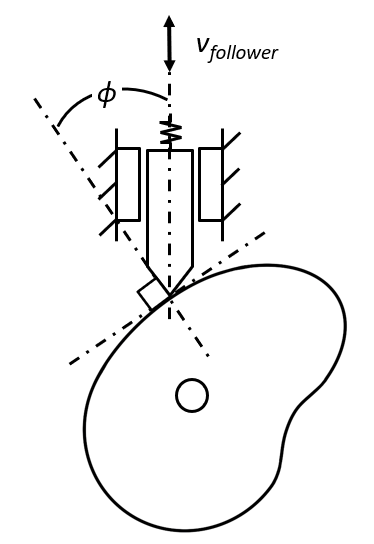
The pressure angle \( \phi \) is defined as the angle between the velocity of the follower and the direction of the axis of transmission. A high pressure angle can cause excessive friction and wear and can even jam the mechanism. The pressure angle should not exceed \( 30^\circ \) for translating followers and \( 35^\circ \) for rotating followers.

Figure 5: Pressure Angle

Motion Programing

The easiest way to design a cam profile is to divide the follower's motion into a piecewise function \( s (\theta) \), whose domain is \( [0^\circ,360^\circ) \). Each subdomain is assigned one of the following three functions:

• Dwell - The follower is maintained at a constant position.
• Rise - The follower is raised to desired position.
• Fall - The follower is lowered to a desired position.

Figure 6: Demonstration of Parts of Motion Program

When designing a cam, the following variables must be considered:

• Displacement - \( s (\theta) \)
• Velocity - \( v (\theta) =\dot{s}(\theta) \)
• Acceleration - \( a (\theta) =\ddot{s}(\theta) \)
• Jerk - \( j (\theta) =\dddot{s}(\theta) \)

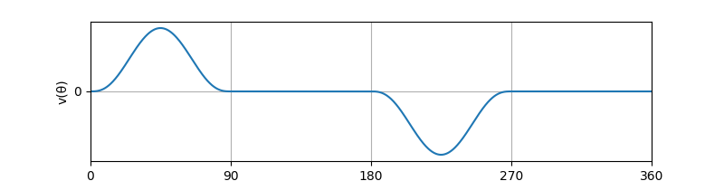
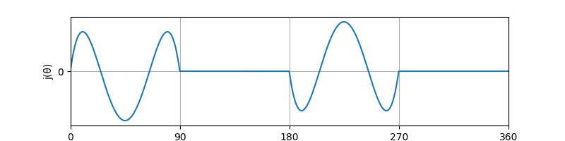
These variables can be represented by plotting their values across the entire surface of the CAM. Since we are plotting Displacement (S), Velocity (V), Acceleration (A), and Jerk (J) we call this an SVAJ plot.

Fundamental Law of Cam Design: When designing a cam, it is critical that the position, velocity, and acceleration of the follower motion are continuous. Additionally, the jerk must be finite because rapid changes in jerk can excite harmonics in the cam system, causing vibrations.

Cam Profiles

The Fundamental Law of Cam Design helps us define boundary conditions for the rise or fall segment. Afterwards, each section can be pieced together to from a whole rotation.

This section includes several cam profile examples, but is by no means an exhaustive list. Each example assumes a rise-dwell-fall-swell cam profile with \( 90^\circ \) for each section. Let us first look at a trapezoidal profile to see why linear functions, though simple, are not a good idea. Think of a trapezoidal rise or fall section as a simple ramp, so the entire \( s (\theta) \) graph looks like a trapezoid. We call this the trapezoidal profile. (Note that in the below equations \( h \) is how high the cam rises and falls)

Figure 7: Trapezoidal Position

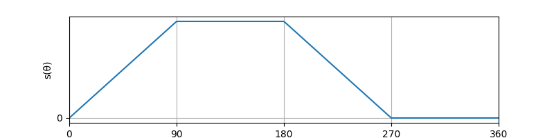
The position function is continuous. But taking the derivative of \( s(\theta) \), we can see that the velocity function is not.

Figure 8: Trapezoidal Velocity

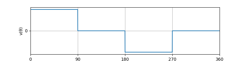
This will result in spikes of infinite acceleration.

Figure 9: Trapezoidal Acceleration

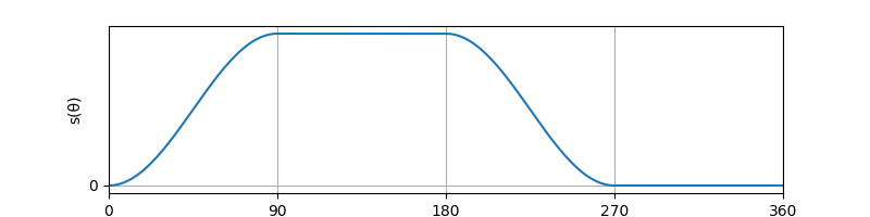
Now, let's enforce continuous velocity boundary conditions where the rise and fall sections meet with the dwell section. One equation that satisfies this is a sine function similar to that of simple harmonic motion, hence we call this the simple harmonic profile. (Note that \( \beta \) is the angular interval of the function. For all following examples, \( \beta=90^\circ \).)

Figure 10: Harmonic Velocity

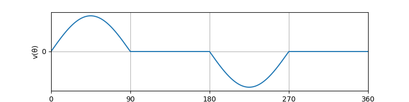
We can find \( s(\theta) \) for the rise section by integrating \( v(\theta) \) and enforcing the boundary conditions \( s(\theta)=0 \) and \( s(\theta)=h \), as shown below. We can also get the profile for the fall section by reflecting the rise portion by reflecting the rise portion across the horizontal axis, then shifting it upwards by \( h \).

Figure 11: Harmonic Position

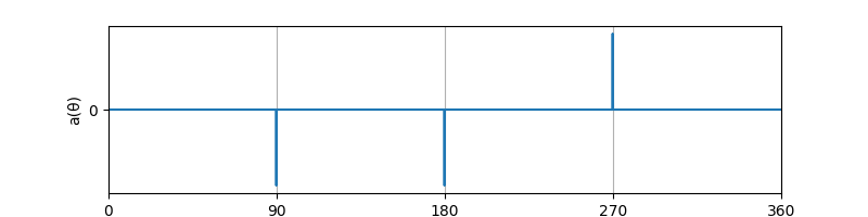
Both \( s(\theta) \) and \( v(\theta) \) are continuous. But when we consider its acceleration function, we can see that it is discontinuous at the section transitions, meaning jerk is infinite at these locations.

Figure 12: Harmonic Acceleration

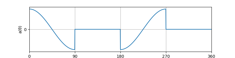
Thus, a better approach to this problem is to design an acceleration function that is continuous and then integrate and apply boundary conditions to get the position and velocity equations. Let's start by prescribing a continuous sinusoidal acceleration function. The coefficient \( 2\pi\frac{h}{\beta^2} \) was found by integrating \( a(\theta) \) with an unknown coefficient then applying boundary conditions \( s(0)=0 \), \( s(\beta)=h \), \( v(\theta)=0 \), \( v(\beta)=0 \), \( a()=0 \), \( a(\beta)=0 \). We call this a Cycloidal profile.

Figure 13: Cycloidal Acceleration

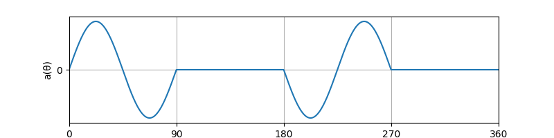
We can integrate to get the velocity and position function and differentiate to get the jerk function.

Figure 14: Cycloidal Position

Figure 14: Cycloidal Velocity

Figure 14: Cycloidal Jerk

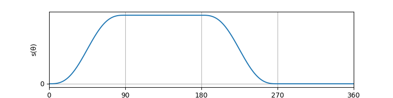
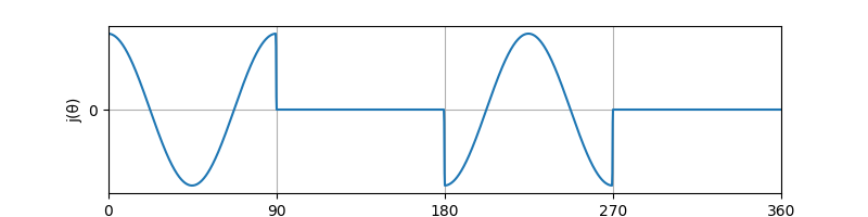
Note that the position, velocity, and acceleration functions are all continuous and the jerk is finite. However, there is still room for improvement. A steep acceleration function can still create large jumps in jerk.

Instead of using trigonometric functions, we can construct a polynomial position function that has continuous jerk and enforce position, velocity, acceleration, and jerk boundary conditions on it. In total, there are 8 boundary conditions \( s(0)=0 \), \( s(\beta)=h \), \( v(\theta)=0 \), \( v(\beta)=0 \), \( a()=0 \), \( a(\beta)=0 \),\( j(j)=0 \),\( j(\beta)=0 \) so our polynomial will be degree 7 (therefore, 8 unknown coefficients).

Solving for coefficients \( C_0...C_7 \) gives us:

Figure 15: Polynomial Position

Figure 16: Polynomial Velocity

Figure 17: Polynomial Acceleration

Figure 18: Polynomial Jerk

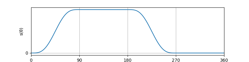
This is known as the 4-5-6-7 polynomial profile. We can also use a similar process to create other profile shapes given a set of boundary conditions.

Cam Profile Selection

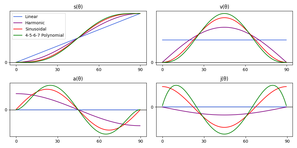
Selecting the right cam profile for your application doesn't depend solely on continuous jerk. For example, if your mechanism has weak joints but is not susceptible to vibrations, you may want to select a cam profile with low peak acceleration (e.g. modified trapezoidal). If you want to smooth out your follower motion, you may want to select a cam profile with lower peak velocity (e.g. sinusoidal). If you want to decrease the pressure angle, you may want to select a cam profile with a less aggressive slope (i.e. harmonic).

The following is a comparison of the rise SVAJ plots of the four profiles covered so far.

Figure 19: Polynomial Jerk

Function Transformation

You may have noticed that the vertical scale has been omitted and the horizontal scale for the rise and fall sections is set arbitrarily at \( \beta=90^\circ \) for all graphs so far. This is because you can achieve any vertical and horizontal scaling from a normalized rise function.

Suppose that we have a normalized rise function, \( s_0(\theta) \), where \( s_0(0)=0 \) and \( s_0(1)=1 \). Using function transformations, we can transform \( s_0(\theta) \) to go from any \( s_0(\theta_i)=h_i \) to \( s_0(\theta_f)=h_f \), where \( \theta_f=\theta_i+\beta \).