Instant Centers Intro

From previous experiences with mechanisms, one may recall that any rigid body has an angular velocity. Furthermore, one may recall that an angular velocity can create a linear velocity according to the equation:

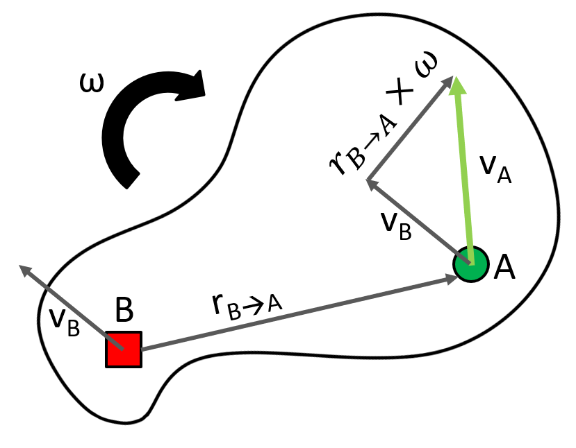
In this figure Where \( A \) is the velocity of the point attached to the rigid body that we are interested in, \( B \) is another point that we know the velocity of on the rigid body, \( r_{b \rightarrow a} \) is the position vector from point \( A \) to \( B \), and \( \omega \) is the angular velocity of the rigid body.

If we look closer at the above equation, we can see that by changing the position of point \( A \), we will change \( r_{b \rightarrow a} \), which will change \( v_a \). This means that for any value of \( v_a \) we can find a position \( A \) that will make the equation hold true. Note: This point may not be on the rigid body. This is okay, we just need to treat the point \( A \) as if it were connected to the same rigid body, even if it is not.

Lets now consider a pair of two rigid bodies. We know that each of these rigid bodies may have its own \( \omega \). However, since we know we can select a point \( A \) so that it can have any velocity, that means that we can find a point where the velocities of both rigid bodies are the same. More precisely, if we know the velocity of point \( B \) on rigid body \( 1 \), and the velocity of point \( C \) on rigid body \( 2 \), we can find point \( A \) such that:

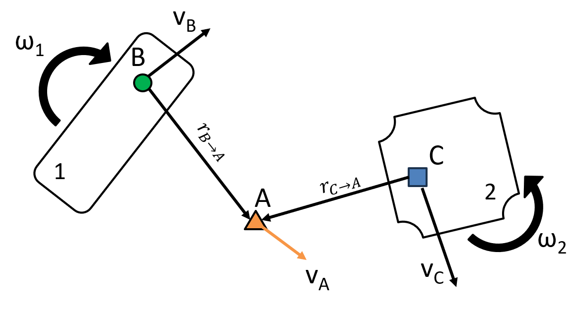
We call point \( A \) where the linear velocities of both rigid bodies are the same the Instant Center, or IC, of these two rigid bodies. This is because at a given instant, we can treat point \( A \) as the center or axis of rotation. The unique properties of instant centers allow us to quickly compute the velocities of different elements in a mechanism.

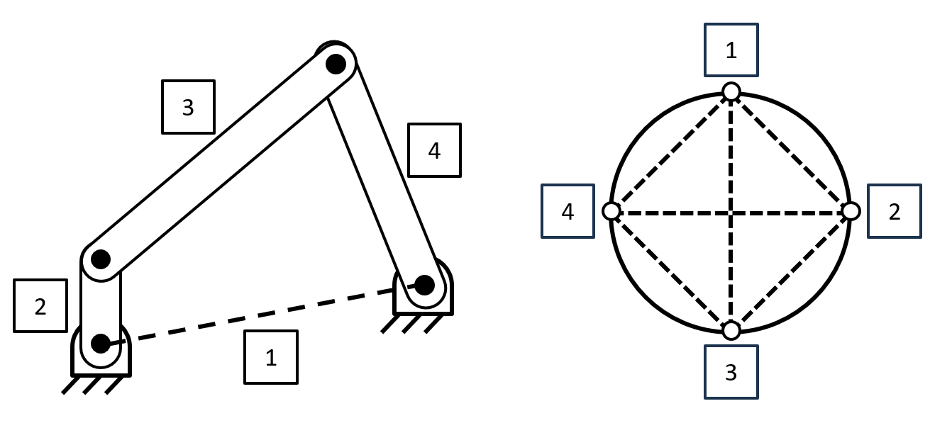
Finding Instant Centers

The first step in using instant centers to compute velocity information in a mechanism is to identify where the instant centers are. We can find an instant center for each pair of rigid bodies in a mechanism. This means that for a mechanism with \( \) links, the total number of instant centers can be computed using the following equation.

Thus, a 4 bar mechanism would have 6 IC's, and a 6 bar mechanism would have 15. It can be easy to overlook or miss an IC. One useful way of keeping track of these IC's is to make use of a simple circle diagram. Begin by drawing a circle, and label points along the circumference, one point for each rigid body in the mechanism. As each instant center is identified, draw a line that connects the two rigid bodies that define that instant center. This creates an easy method to keep track of IC's and ensure that none are missed.

Once we know the number of instant centers we are looking for, there are a few simple rules that will help us find all of them.

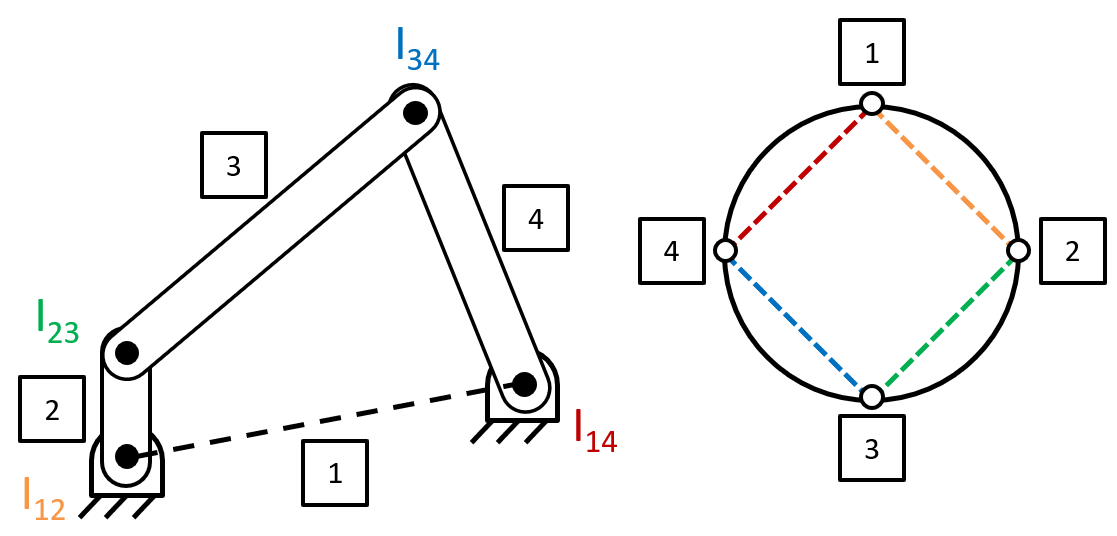
Rule 1: Each pin joint is an IC

A pin joint constraints two or more rigid bodies to have the exact same linear velocity at a point, even if they have different angular velocities. Thus, a pin joint creates an instant center between those two objects

Rule 2: Kennedy's Theorem

3 bodies that are in the same plane will have their instant centers lie along a line.

Commonly called Kennedy's theorem, this rule is often used to find the instant centers between rigid bodies that are not in contact with one another. From our number of instant centers equation, we know that 3 bodies will have \( \frac{3(3-1)}{2}=3 \) IC's. If we can find two of them, then we know that the third instant center must also be on the line that passes through the previous two.

If we are able to do this process with another set of instant centers, we can get two different lines that the instant center must lie on. Since the instant center must be on both of these lines, it must exist at the intersection of the two lines.

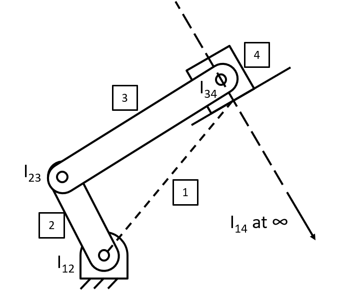
Rule 3: Sliding Joints

The IC for a sliding joint is located at an infinite distance away from the mechanism, perpendicular to the sliding direction.

In a sliding joint, there is no rotation, so how can two objects ever have the same linear velocity? By placing the instant center at infinity, we can treat the motion of the slider as a having a very small omega, and a very large radius, giving us an approximately linear motion. As the radius goes to infinity, the velocity will approach perfectly linear motion.

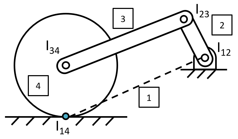
Rule 4: Rolling without Slipping

For two bodies in rolling contact without slipping, the contact point is their IC.

If two bodies are rolling without slipping, they must have the same velocity at the contact point, meaning that this point is an instant center.

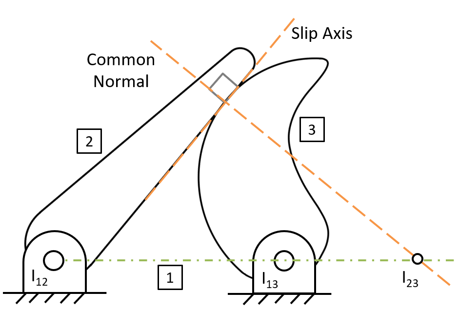
Rule 5: Rolling with Slipping

For two bodies in rolling contact with slipping, which we can think of as a combination of rolling (IC at contact point) and sliding (IC at infinity). As a result, we can deduce that the IC lies on a line normal to their plane of contact. Additionally, the IC lies on the same line as their common centers of rotation according to Kennedy's theorem. The third body can be thought of as the ground link, hence the pivots are two instant centers.

Using Instant Centers

Now that we have a method to reliably find the instant centers of a mechanism, we can use these instant centers to find the velocities of different elements of the mechanism.

We can use instant centers to easily find the ratio of velocities between different elements. Any given point \( p \) can only have one translational velocity, \( v_p \). However, at an instant center, we know that these translational velocities are equivalent for two different rigid bodies.

Thus, if we have velocity information for one element in a mechanism (angular or translational) we can use that to find velocity information for other elements.

We can look at the following example to see this in more detail

1. Begin by listing known information. In this case, we know the link lengths of a mechanism, as well as the angular velocity of the crank.
   
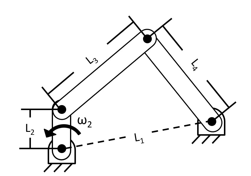
2. Next, compute all of the instant centers on the mechanism.
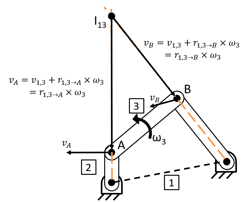
3. We then can consider the crank of the mechanism. We know that the pin between the crank and ground is an instant center. Since the ground link has a velocity of 0 everywhere, the crank will have a velocity of 0 at that location. Let's call the crank body 2, and the ground link body 1.
4. Then, select another grounded linkage. This is the link that we will analyze. Let's call that body 3. Body 1 and body 3 will share an instant center, which we will call \( A \).
5. Using \( v_a=v_{IC_{1,2}}+r_{IC_{1,2} \rightarrow a} \times \omega_2 \) we can substitute in for \( v_{IC_{1,2}}, r_{IC_{1,2} \rightarrow a} \) and \( \omega_2 \) to find \( v_a \).
   
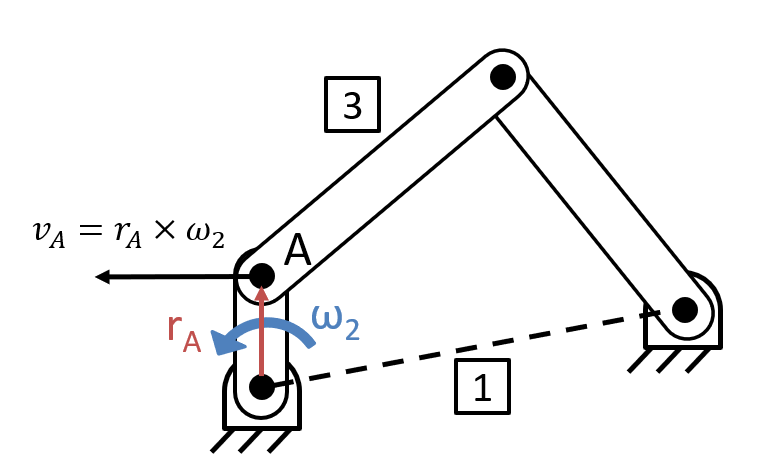
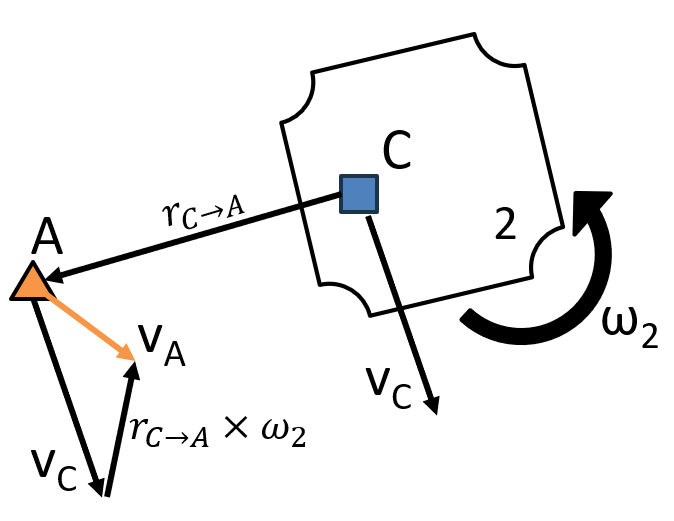
6. We can reuse the above equation, but instead consider that point \( A \) is also attached to body 3. Thus, we could consider the velocity of point \( A \) as coming from the rotation of body 3 rather than the rotation of body 2. We would write this equation as \( v_a=v_c+r_{c \rightarrow a} \times \omega_3 \).
7. The biggest issue here is that we do not know where to place point \( C \) so that we know its velocity. If we place it at point \( A \), the radius will be 0, and we will be unable to compute \( \omega_3 \). However, there is another location where we know the velocity of a point on body 3. If we consider \( IC_{1,3} \) we know that the ground has a velocity of 0 everywhere. Thus, at \( IC_{1,3} \), the ground and body 3 have the same speed, 0.
8. This allows us to write \( v_a=0+r_{IC_{1,3} \rightarrow a} \times \omega_3 \). Since we know all of these values except \( \omega_3 \), we can then solve for \( \omega_3 \).
9. Now that \( \omega_3 \) is known, we can compute \( V_b \), and \( \omega_4 \). Additionally, this procedure can be repeated to find the velocities of all links in a mechanism.
   

Using this style of procedure, we can use instant centers to compute the velocities of different elements of any mechanism.