Graphical Linkage Sythesis Intro

Kinematic synthesis (also known as mechanism synthesis) is the act if designing mechanisms with a specified motion to perform a specific task. Kinematic synthesis often follows this procedure:

1. Define desired motion. Does your mechanism need to open and close a lid or mimic the way an animal walks? What is motion you are trying to achieve?
2. Choose the mechanism type. Will it consist of a crank-rocker, a slider-crank, or some other type of mechanism?
3. Specify the geometry. How long will the links be? What types of joints will be present and how many?
4. Check for undesirable behaviors. Is there a toggle position or a change point in the motion of the mechanism?

Before starting to design a mechanism, it is always encouraged to research existing solutions. One can often adapt an existing design to fit the given specifications by understanding similar problems and the mechanisms used to solve them. There are two main ways to generate or adapt linkages: path and position generation.

Path Generation

The goal of path generation is to make a point follow a predefined path. The point of interest is almost always on a coupler linkage. Cranks will always trace circles, rockers will trace arcs, and sliders trace straight lines which are uninteresting when trying to create a mechanism that follows a complex path.

There are two approaches to path generation: the algebraic approach and using lookup tables. The algebraic approach is very labor intensive and involves finding the zeros of a multidimensional high order polynomial that increases in order as the number of linkages increases. This approach is beyond the scope of this course. A far better approach is to utilize lookup tables that show the path traveled by a coupler point and how the path changes as each linkage changes in length.

The four bar linkage shown below is a simple model that is used to show how lookup tables can be used. In this linkage \( L_1 \) is the ground linkage while \( L_2 \) is the crank. \( BP \) represents the measurement from one joint to the coupler point \( P \). The angle between the coupler \( L_3 \) and link \( BP \) is represented as \( \gamma \), which is known as the offset angle. By changing link lengths and angle gamma, there are many position paths that the coupler point \( P \) can travel.

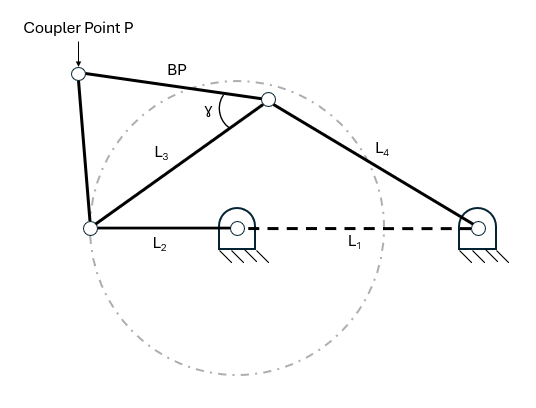
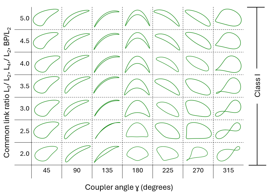
To simplify coupler curve tables, common ratios between linkage lengths are established. \( L_1/L_2 \) is known as the ground link ratio and \( L_3/L_2 \) is the coupler link ratio. \( L_4/L_2 \) is the output link ratio and \( BP/L_2 \) is called the offset link ratio. The table below shows different coupler curves for four-bar linkages where the coupler link, output link, and offset link ratios are all equal. The x-axis shows the offset angle (also known as the coupler angle), while the y-axis shows the common link ratio. Once you choose a desired path, you can read the coupler angle and common link ratio to build a mechanism that follows that exact path.

If you want to change the length of a single link, there are additional tables for different links that can be used to select different types of motion.

Position Generation

Position generation focuses on a link following a prescribed position. In this case, the orientation of the link is also considered when generating the system. This is a very visual process of synthesis which involves drawing out your system. This section will go into a few different methods for using position generation. In order to follow along, you will need a compass, straight edge, and writing device. More complex mechanisms may also require a protractor.

Bisecting a Line with a Compass

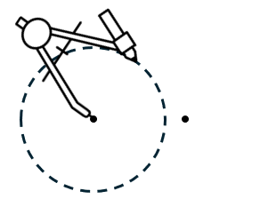
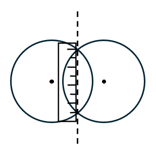
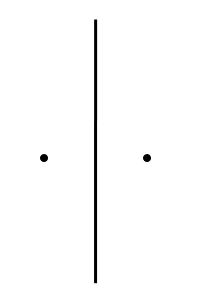
One of the most important fundamental skills for position generation is the ability to construct a perpendicular bisector for a line.

1. Draw two points. Using your compass, draw a circle with a radius that is a little larger than halfway between the two points.

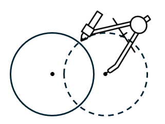
2. Carefully pick up your compass and move it to rest on the other point without changing the radius. Draw another circle between the two points. If you did it right, there should be two intersecting points on the arcs.

3. Line up a ruler with the two intersecting points and draw a straight line.

4. Erase your arcs and you are left with a line that perfectly bisects the two points.

Two Position synthesis: Crank Output

One of the most common position generation problems is two-position synthesis. In this problem, the goal is to select link lengths and point positions that will move the rocker in a crank-rocker linkage from one position to another. Crank output position synthesis is a good choice if you desire your linkage to follow the path of an arc.

1. Draw the desired start and end position for a rocker.

2. Bisect the start and end points. This will represent the rocker's middle position.

3. Draw a straight line connecting the start and end point of the rocker. Choose a point where you want the ground position of your crank to be.

4. Using the distance between the start and the bisecting line as your radius, draw a circle around the ground position of your crank. Place a joint on the circle and connect the ground to your new joint to create your crank.

5. Once you draw in your rocker, you are finished!

Two Position synthesis: Coupler Output

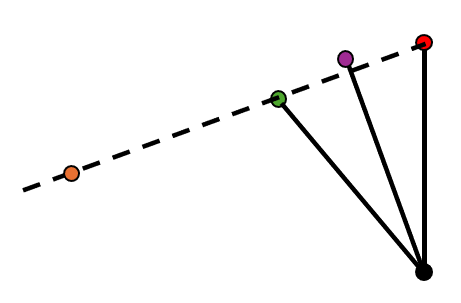
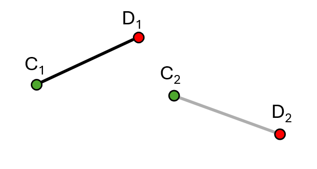
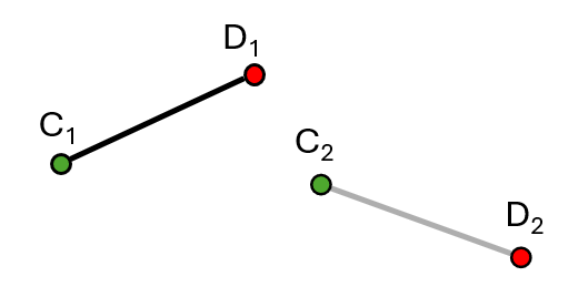
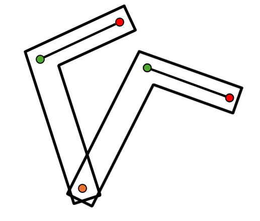
A slightly more complex challenge arises when the goal is to create a mechanism that will move the coupler of a four bar linkage from one position to another.

1. Choose the start and end position of your coupler. In this instance, the start position is labeled with the subscript 1 while the end position is labeled with the subscript 2. Therefore, joint \( C_1 \) is the start position while joint \( C_2 \) is the end position.

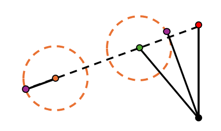
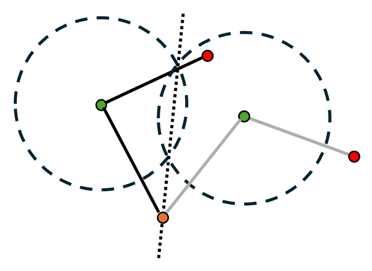
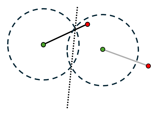
2. Bisect one of the start and end pairs of joints (in this case \( C_1 \) and \( C_2 \)). Choose a position along this line to place a ground joint. This will form one of the linkages connecting to the coupler.

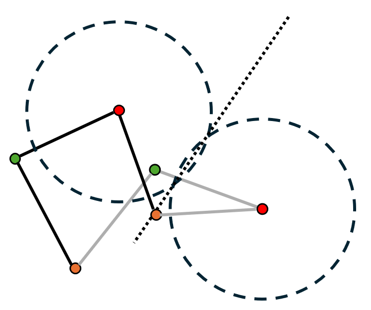
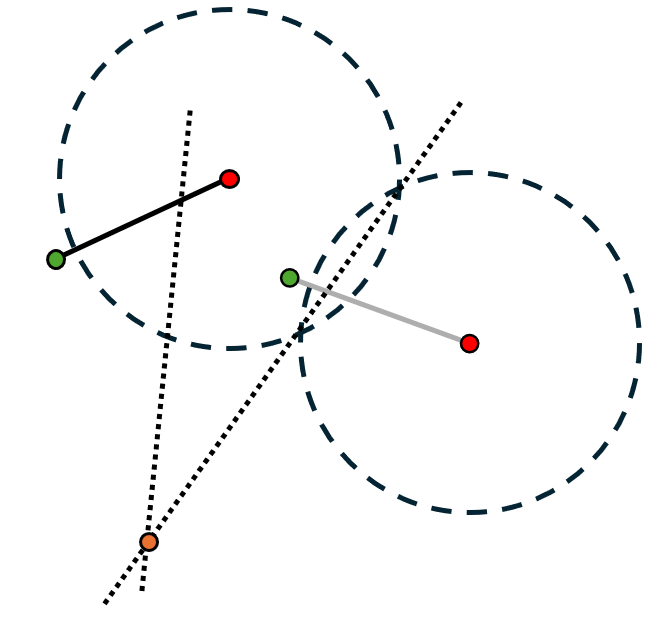
3. Bisect the other pair of start and end joints. Draw another ground point anywhere along the line. This will be the last joint in the four bar linkage.

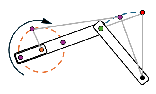
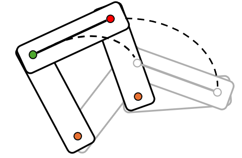
4. Erase all bisecting lines and draw your linkages. You have now completed coupler output synthesis!

Rotopole Synthesis

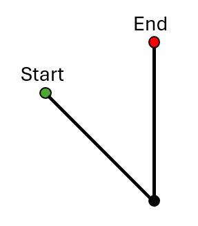
Another approach to the previous two position synthesis problem is to extend the rocker and use it to move between the two positions. This type of mechanism is called a Rotopole.

1. Start with your two desired linkage positions.

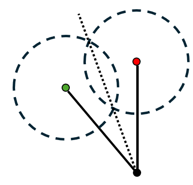
2. Similar to coupler output synthesis, bisect one of the start and end pairs of joints (in this case \( C_1 \) and \( C_2 \)).

3. Bisect the other pair of start and end joints. The place where the two bisecting lines intersect is where the ground joint will be placed.

4. Connect your linkage to your ground joint using one linkage and you are left with a rotopole.

Dyad Driver

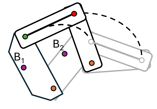
When designing the rotopole, we did not consider the crank or coupler. Fortunately, we can design these links to move the rocker the proper amount. The process of adding a crank and coupler to an existing mechanism (Whether it is a rotopole or other rocker) to move it the proper amount is called adding a "dyad driver".

1. Start with your rotopole or rocker mechanism and choose a point on the already existing linkage. This has been labeled \( B_1 \) for the starting position and \( B_2 \) for the ending position.

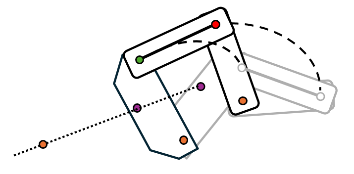
2. Draw a straight line connecting the start and end position of the chosen point. Extend this line out of the way of the mechanism's motion. Choose a point on this line to place the ground joint for the crank.

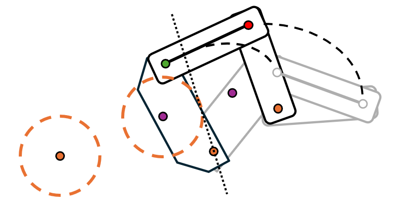
3. Bisect the two chosen points (\( B_1 \) and \( B_2 \)). Use the distance between one of the points as the radius of the crank.

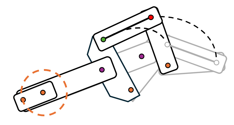
4. Create the crank linkage and add a linkage to attach the coupler to the mechanism. Your dyad driver is now complete.